ExceLab Primer
ExceLab solver functions are just like standard native Excel Math Functions except that they also take formulas as input and solve calculus problems.
For example, if you needed to compute the square root of a number stored in A1, you would use the SQRT math functions in a formula like this
=SQRT(A1)
Like wise, to integrate a formula stored in A1 with respect to X1 between 1 and 2, you use the QUADF calculus function in a formula just like this
=QUADF(A1, X1, 1, 2)
Or, to solve an ODE system, you use an ode solver function like IVSOLVE in a formula like this
=IVSOLVE(Y1:Y3, X1:X3, {0,1})
It is that simple!
Some calculus functions like QUADF compute a single value and are evaluated in a single cell. Other calculus functions like IVSOLVE compute an array of results and must be evaluated as array formula in an allocated range of cells.
You can use the functions individually to solve many calculus problems including interpolation, integrals, derivatives, nonlinear and differential equations. You can also combine the calculus functions with Excel Solver to effortlessly solve many advanced optimization problems including optimal control and parameter estimation.
☞ If you are familiar with Excel, you can hit the road running with ExceLab calculus functions. Jump to the Examples.
☟ If you are new to Excel, spend a few minutes to familiarize yourself with Excel and the following essential skills.
The calculus functions are designed to operate in two modes: a silent mode, where only standard Excel errors are returned like #VALUE!, and a verbose mode, where the
function may display an informative error or warning message alert in a popup window. It is recommended to work in the verbose mode when setting up a problem but to switch to
a silent mode when running an optimization problem with Excel Solver to suppress error popup windows during the optimization.
You can switch between any of the following three modes by evaluation the VERBOSE function with a proper integer flag in any cell in the workbook as described below:
Standard Excel errors
In this mode the solver returns a standard Excel error value such as #VALUE! or #DIV/0!. To activate this mode evaluate the formula=VERBOSE(0)Text error messages
In this mode the solver returns a text value in case of error instead of the numerical result. To activate this mode evaluate the formula=VERBOSE(1)Windows error dialogs
In this mode the solver displays a popup windows dialog box with the error message. Manual dismissal of the error window is required to continue. To activate this mode evaluate the formula=VERBOSE(2)
The default mode is set to Text error messages.
Sometimes it is convenient to work with raw addresses like X1, to quickly define a function. Other times it is more convenient to assign a name to a cell (or range of cells), and refer to the cell by its name. The advantages of working with named variables:
You can organize/group your variables and place them where you want in the spreadsheet.
Your formulas become easier to read and find errors.
Your named variables are automatically locked. Excel will not increment them when you perform an AutoFill operation.
There are two ways to assign a name for a cell:
-
Using Address Box
Click on a cell (or highlight a range of cells) on Sheet1, then enter your desired name (e.g., MyCell) in the address box and click enter.
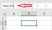
Be aware that name you have just defined this way becomes a global name in the whole workbook which is not always a good idea. If you use MyCell anywhere in the workbook it will always reference Sheet1!B2.
-
Using Name Manager
To restrict the scope of a named variable to the worksheet it belongs to, use the Name Manager which you invoke from the Formulas Tab to name the variable.
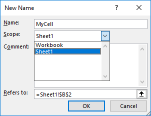
MyCell is now defined on Sheet1 only. You can define MyCell again on a different sheet and use it without cross-sheet interference.
It is a good convention to insert a label next to your named variable cell like this
| A | B | |
| 1 | ||
| 2 | MyCell | 1 |
Note. ExceLab 365 and Google Sheets support a new spill feature which allows you evaluate an array formula like a standard formula by pressing Enter and the array result will spill into neighboring cells. This feature is not supported in ExceLab 7.
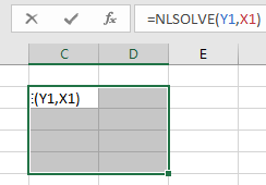
If a function computes a single number such as the native SQRT (square root), or QUADF (integral solver), you would evaluate it in a standard formula in a single cell. On the other hand, of a function computes an array of numbers such as the native MINVERSE (matrix invers) or IVSOLVE (ODE solver), then you must evaluate it in a pre-allocated range of cells big enough to hold the expected result. Some functions like the interpolation functions, can be evaluated both as a standard formula in a single cell (if you are interpolating at a single point), as well as an array formula in a range (if you are interpolating at a vector of points at once which could be more efficient than using AutoFill operation to accomplish the same result). Similary NLSOLVE (equations solver) can be evaluated as a standard formula in a single cell (if you are solving for one variable), or as an array formula in a range (if you are solving for multiple variables at once).
To evaluate an array formula, you do the following:
Highlight the array of cells which will hold the result to select it.
While the array is selected, click in the formula bar and enter your formula as you would normally do.
-
While still in the formula bar, press Ctrl+Shift+Enter at the same time.
Another way to evaluate the array formula is to:
Enter the formula in one cell first and evaluate it with Enter. Ignore any error or warning.
Enlarge the cell into an array.
While the array is selected, click in the formula bar and press Ctrl+Shift+Enter at the same time.
Once you have evaluated an array formula in a selected array, you cannot shrink the array but you can enlarge it. The only way to shrink the array is to delete it and re-enter your formula!
Reference Types
Formulas and variables are always passed by reference either by raw address or by assigned name.
When passing multiple formulas or variables into one argument:
If the cells are contiguous, you can pass the range address for example, A1:A4 or its assigned name.
-
If your formulas or variables are in diconnected cells, use Excel union operator, (Ref1,Ref2,Ref3,..), to combine them into one reference. For example, we can combine the variables (T1,X1,U1:U3) into one reference and pass it in a single argument to a solver.
A formula can have explicit or implicit dependence on variables via dependence on other nested formulas. However, you always pass the root (top) formula and the variables to any calculus function.
Value Types
You can pass value types like numbers and strings directly as arguments or by reference.
-
Often, you need to pass a vector of values in one argument which you can pass either by reference or by using Array Constant syntax. For example, the two formulas below are equivalent:
- Using array constant syntax
=QUADF(A1,X1,0,1,{"ALGOR","QAGS";"RTOL",0.0001})- Using array reference
=QUADF(A1,X1,0,1,B1:C2)
C B 1 ALGOR QAGS 2 RTOL 0.0001
Note that a string literal must be enclosed by double quotes when entered by value but no quotes are needed if entered by reference.
Frequently, you want to repeat a computation for a sequence of values, for example, interpolating or computing the derivative at a vector of pre-defined points, say X1:X50. Excel AutoFill feature comes very handy, where you define a starting formula, then drag it down to generate new calculations with auto updated parameter values. During the Autofill operation, it is important to lock the function parameters that should not be altered, and only allow Excel to increment the variable parameter such as an interpolation or differentiation point. To lock a function parameter, you can use one of two methods:
Assign names to the ranges or cells you don’t want Excel to increment, and pass the names instead of the raw addresses.
-
Use the locking operator, $, to lock a row, column or both of any range or cell address. For example, $A$1 locks both the column to A and the row to 1. Excel will not increment $A$1 during an autofill operation. Similarly, you can lock a range of cells, for example, $A$1:$B$10.
Your interpolation formula may look like this:
=INTERPXY(xVector, yVector, X1) or
=INTERPXY($A$1:$A$50, $B$1:$B$50, X1)
Now if you drag this formula, Excel will invoke INTERPXY, at a new value of X1, X2, X3 … while holding the first two parameters constants.
Excel gives precedence to the unary negation operator, -, over the exponent operator, ^ which may lead to undetectable errors in your formulas. For example, Excel evaluates the formula =-X1^2 as =(-X1)^2. Try it! Your intention may have been to do -(X1^2) instead. A simple fix for this is to either use parenthesis or to use the native POWER function like =-POWER(X1,2).