Computing Numerical Derivative of a Function in Excel

Syntax

`=DERIVF(f, x, p, [options])`

Description

Use DERIVF to compute first or higher order derivatives of a function f(x) at x=p using highly accurate adaptive algorithm. With optional arguments, you can specify a higher derivative order, as well as override the default algorithm parameters.

\frac{d^{n} f (x)}{d x^{n}}

DERIVF can be nested to compute partial derivatives of any order.

\frac{\partial}{\partial z} \frac{\partial}{\partial y} \frac{\partial}{\partial x} f (x, y, z)

Inputs

Required Inputs

f a reference to the function formula.

If your function is too complex to represent by nested formulas, you can code it in a VBA function (see Example 3).

x a reference to the variable of differentiation.

p the point at which to compute the derivative.

Optional Inputs

n the derivative order. You can enter an integer number from 1 to 4. Default is 1.

ctrl a set of key/value pairs for algorithmic control as detailed below.

Description of key/value pairs for algorithmic control

Relative error control

Key	RTOL
Admissible Values (Real)	`> 0`
Default Value	(0.00001 for (n = 1) 0.0001 for (n = 2) 0.001 for (n = 3) 0.01 for (n = 4)
Remarks	Convergence is a function of several factors including function metric. Setting RTOL too small may prevent successful convergence.

Starting step size for Ridders' algorithm

Key	INITSTEP
Admissible Values (Integer)	`> 0`
Default Value	0.05
Remarks	This parameter is very influential. Try different small and large values when encountering convergence difficulties.

Iterations control

Key	ITRNMAX
Admissible Values (Real)	>= 3
Default Value	50
Remarks	Sets an upper bound on the maximum size of the generated Neville' tableau by Ridders' algorithm.

Examples

Collapse all examples

Example 1: Computing first and higher-order derivatives of a function

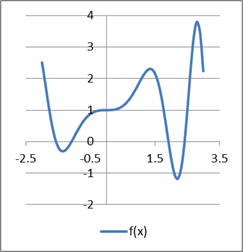
Consider the function:

$f (x) = x sin (x^{2}) + 1$

The analytic derivatives of f(x) up to order four are:

$f^{'} (x) = sin (x^{2}) + 2 x^{2} cos (x^{2})$

$f^{''} (x) = 6 x cos (x^{2}) - 4 x^{3} sin (x^{2})$

$f^{'''} (x) = 6 cos (x^{2}) - 8 x^{4} cos (x^{2}) - 24 x^{2} sin (x^{2})$

$f^{''''} (x) = 16 x^{5} sin (x^{2}) - 80 x^{3} cos (x^{2}) - 60 x sin (x^{2})$

We compute the numerical derivatives of at x = 0 and at x = 1 for orders 1 to 4 and compare them to the analytical values shown in column B of the tables below:

At `x=0`

	A
1	=X1*SIN(X1^2)+1
2	=DERIVF(A1,X1,0)
3	=DERIVF(A1,X1,0,2)
4	=DERIVF(A1,X1,0,3)
5	=DERIVF(A1,X1,0,4)

⇒

	A	B
1	1	1
2	3.18603E-15	0
3	0	0
4	6	6
5	1.27896E-15	0

At `x=1`

	A
6	=DERIVF(A1,X1,1)
7	=DERIVF(A1,X1,1,2)
8	=DERIVF(A1,X1,1,3)
9	=DERIVF(A1,X1,1,4)

⇒

	A	B
6	1.922075597	1.922075597
7	-0.124070104	-0.124070104
8	-21.27590825	-21.27590825
9	-80.24890792	80.24890780

Example 2: Computing mixed partial derivatives of a 2-dimensional function

Consider the partial derivative:

$\frac{\partial}{\partial y} \frac{\partial}{\partial x} cos (x, y) = - sin (x y) - x y cos (x y)$

We compute the partial derivative of cos(xy) at (π,π) by nesting DERIVF and compare the result with the analytical value shown in B3 below:

Partial derivative at `(π,π)`

	A
1	=COS(X1*Y1)
2	=DERIVF(B1,X1,PI())
3	=DERIVF(B2,Y1,PI())

⇒

	A	B
1	1
2	0
3	9.3394486379	9.3394486379

Example 3: Computing derivative of a user-defined VBA function

We demonstrate how to compute the derivative for a user defined VBA function with DERIVF. You can define your own VBA functions in Excel which is quite powerful when your function is difficult to define with standard formulas. For illustration, we compute the derivative for

$log (x + 1)$ , at x=2.

VBA is supported in ExceLab 7.0 only. ExceLab 365 which is based on cross-platform Office JS technology is not compatible with VBA

Solution

Open Excel and start VBA Editor by pressing Alt+F11
Insert a Module from the Insert Tab, then code the following function:
Save the workbook with the extension xlsm (macro enabled) and close VBA editor
In Sheet1, define your function formula as shown in A11.We pass the differentiation variable and any other parameters the VBA function expects.

Compute derivative at `x=2`

	A
11	=vbMyFunction(X1, 1)
12	=DERIVF(A11,X1,2)

⇒

	A
11	0
12	0.333333

Your VBA function name must be prefixed with "vb" to be used with ExceLab solvers.

X1 is just a dummy variable for the function and its value is ignored.

Algorithms

DERIVF implements Ridders' method which uses an adaptive step to produce a much higher precision than a simple finite differencing method with a fixed step. It employs Neville' algorithm and polynomial extrapolation to drive the step size to zero within machine accuracy.

The starting step size for Ridders's algorithm is an important parameter that can aid successful convergence of the algorithm. You can override the default value of this parameter using the control key INITSTEP (for example, DERIVF(A1, X1, P1, 1, {"INITSTEP",0.1})). The starting step size need not necessarily be small but rather should scale with a range around the point p over which the function changes noticeably. Ridders' method attempts to drive the step size to zero by polynomial extrapolation using Neville' algorithm.

References

Ridders, C.J.F. Advances in Engineering Software. Volume 4, No. 2, pp 75-76. (1982)

ExcelWorks LLC

Computing Numerical Derivative of a Function in Excel

Syntax

=DERIVF(f, x, p, [options])

Required Inputs

Optional Inputs

At x=0

At x=1

Partial derivative at (π,π)