Solving boundary value problems in Excel

Syntax

`=BVSOLVE(eqns, vars, bcs, domain, [options])`

Description

Use BVSOLVE to solve a boundary-value ODE or DAE system in the form: (the system can have as many equations as needed)

Example:

\frac{d y_{1}}{d x} = f_{1} (x, y_{1}, y_{2}, y_{3})

\frac{d y_{2}}{d x} = f_{2} (x, y_{1}, y_{2}, y_{3})

With optional one or more algebraic equations:

0 = g_{1} (x, y_{1}, y_{2}, y_{3})

Boundary Conditions

To complete description of the problem, boundary conditions implicating the differential variables are required. General nonlinear boundary conditions can be specified at any location within the the system spatial domain [x_s, x_e].

Inputs

Required Inputs

eqns a reference to the system formulas (f₁, f₂,..,g₁,..).

vars a reference to the system variables in the following order (x, y₁, y₂,.. ).

Optional. You can define starting guess for (y₁, y₂,.. ). The guess can be a constant or a function of x.

Variables order must be consistent with equations order. For example, given this order (x, y₁, y₂,.. ) implies dy₁/dx = f₁, dy₂/dx = f₂ and so forth.

Enter as a reference to a range. for Example, X1:X3. If your variables are not in a contiguous range, say X1, Y1, Y2, you can combine them and pass them as one reference as follows:
Use range union syntax (X1, Y1, Y2) . Supported in ExceLab 7 only
Use array constant syntax {X1, Y1, Y2}. Supported in Google Sheets only
ExceLab 365 supports only contiguous range input for multiple variables but, for convenience, will accept passing noncontiguous variables as string value "(X1,Y1,Y2)"

bcs A reference to a 2-column array defining the boundary conditions. The first column specifies boundary conditions points, and the 2nd column specifies corresponding boundary condition formulas. The boundary conditions points must be ordered from left to right.

Boundary condition points may be repeated if multiple boundary conditions are specified at the same location.

A boundary condition formula is arranged with respect to zero on one side. For Example, suppose that the boundary condition (BC) at x₀ is y₁= y₂+1, then the BC formula may be defined as =Y1-Y2-1.

domain a vector defining the start and end values for the spatial domain. Additional optional data controls the output spatial values in the computed solution as described below.

Domain formats for solution output control

Format	Remarks
{`x_s, x_e`}	The domain [`x_s, x_e`] is divided uniformly according to the number of allocated rowsin the output array.
{`{x_s, x_e, ndiv`}	The domain [`x_s, x_e`] is divided uniformly into `ndiv` subintervals.The allocated output array must have sufficient rows to hold the result.
{`x_s, x₁, x₂, .., x_e`}	Solution results are reported for the supplied values only. The allocated output array must have sufficient rows to hold the result.

Optional Inputs

m the number of algebraic equations for a DAE system.

For a DAE system, algebraic equations and variables should be listed last in eqns and vars.

rtol relative error tolerance. you may specify a fixed value for all variables, or supply vector of tolerances for each variable in vars. Default is 1.0e-4.

ctrl a set of key/value pairs for algorithmic control as detailed below.

Description of key/value pairs for algorithmic control

Algorithm Control

Key	MAXMESH
Default Value	1000 (Integer)
Remarks	Sets an upper bound on the mesh size for the spatial domain.

Key	INITMESH
Default Value	7 (Integer)
Remarks	Sets the initial mesh size which is refined adaptively during iterations.

Key	KORDER
Admissible Values (Integer)	2 ≤ KORDER ≤ 7
Default Value	4
Remarks	No. of collocation points per mesh subinterval. A higher value will increase computational cost.It may help with a highly oscillating system.

Key	LINEAR
Admissible Values (Boolean)	True or False
Default Value	False
Remarks	Set to TRUE if the problem is linear with linear boundary conditions

Key	ERROREST
Admissible Values (Boolean)	True or False
Default Value	False
Remarks	Set to true to report global error estimates for the differential variables in the solution output array.The last row of the allocated output array will be reserved for the error estimates.

Jacobian Approximation

Key	JACSTEP
Admissible Values (Real)	`0 < JACSTEP < 0.1`
Default Value	The default step is computed dynamically based on machine accuracy, preset limits and function metric. For an order(1) function it is approximately 1.0e-8.
Remarks	The default value generally produces accurate approximations; however relaxing the default value may aid convergence on some problems with unknown Jacobian such as parameterized problems.

Key	JACSCHEME
Admissible Values (Integer)	1 for First order Euler forward scheme 2 for Second order Euler forward scheme
Default Value	1
Remarks	First order scheme is generally sufficient.

Output Format

BVSOLVE is evaluated as an array formula in an allocated range of the spreadsheet. It computes and displays a formatted solution as illustrated in Figure 1 for a system with two state variables and a spatial domain [0 ,1]. The first column displays the spatial points, and the subsequent columns display the corresponding values of the state variables.

Figure 1: BVSOLVE formatted output
	A	B	C
1	x	y1	y2
2	0	`y1(0)`	`y2(0)`
3	0.1	↓	↓
4	0.2
..	↓
12	1	y1(1)	y1(1)
13	Rel. Error	error y1	error y2

When allocating a range for BVSOLVE, the following rules apply:

The number of allocated columns should match the number of variables.

The number of allocated rows is arbitrary. It determines the increment for the domain subdivisions (only for display purpose).
You can customize the output spatial points using any of the following formats in argument number 5.

Format	Remarks
{`x_s, x_e`}	The domain [`x_s, x_e`] is divided uniformly according to the number of allocated rowsin the output array.
{`{x_s, x_e, ndiv`}	The domain [`x_s, x_e`] is divided uniformly into `ndiv` subintervals.The allocated output array must have sufficient rows to hold the result.
{`x_s, x₁, x₂, .., x_e`}	Solution results are reported for the supplied values only. The allocated output array must have sufficient rows to hold the result.

If the control key ERROREST value is set to True (see examples below), the last row in the allocated output array will display the estimated maximum global error for each variable.

Examples

Collapse all examples

Example 1: Nonlinear boundary value problem

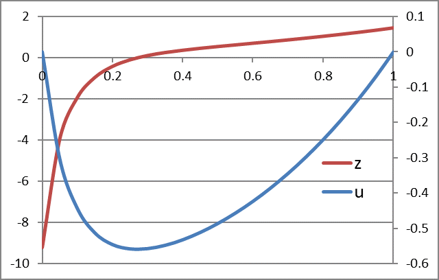
Consider the following 2nd-order nonlinear differential equation in the spatial domain [0,1]

ϵ u^{''} = - e^{u} u^{'} + \frac{1}{2} π \sin (\frac{1}{2} π x) e^{2 u}, 0 \leq x \leq 1

with end points boundary conditions:

u (0) = 0, u (1) = 0

Solution

Using standard substitution technique we convert the 2nd-order equation to two 1st-order equations

\frac{d u}{d x} = z

\frac{d z}{d x} = \frac{1}{ε} (- e^{u} z + \frac{1}{2} π \sin (\frac{1}{2} π x) e^{2 u})

Working with the named variables x, y, z, and eps for cells B2:B5, we define the system equations and boundary conditions as shown in Table 1 below. The colored ranges represent the required input arguments to BVSOLVE. They are: the RHS-side formulas in B7:B8, the selected system variables B2:B4 (named x, y, z,), and the boundary conditions matrix C2:D3.

Table 1
	A	B	C	D
1		Variables	BCs
2	x		0	=u
3	u		1	=u
4	z
5	eps	0.01
6		Equations
7	du/dx	=z
8	dz/dx	=(-EXP(u)z+0.5PI()SIN(0.5PI()x)EXP(2*u))/eps

Next, we evaluate the array formula =BVSOLVE(B7:B8, B2:B4, C2:D3, {0,1}, , , {"ERROREST", True}) in an allocated array G4:I25 and obtain the solution shown in Table 2 below.

Note that we skip over optional parameters 5 and 6 and pass the key ERROREST in parameter 7 to report global error estimates in the last row of the output array.

The obtained result is plotted in Figure 1.

Table 2
	G	H	I
4	x	u	z
5	0	0	-9.22395
6	0.05	-0.3043492	-3.93625
7	0.1	-0.44424441	-1.92551
8	0.15	-0.51353621	-0.95066
9	0.2	-0.54647914	-0.41601
10	0.25	-0.55866051	-0.09636
11	0.3	-0.55796756	0.110589
12	0.35	-0.5486075	0.256436
13	0.4	-0.53287428	0.368873
14	0.45	-0.51201677	0.463304
15	0.5	-0.48669581	0.548502
16	0.55	-0.45723449	0.629561
17	0.6	-0.42375759	0.709506
18	0.65	-0.38627075	0.790212
19	0.7	-0.34470297	0.872914
20	0.75	-0.29893093	0.958517
21	0.8	-0.24879048	1.047768
22	0.85	-0.19408162	1.14137
23	0.9	-0.13456902	1.240042
24	0.95	-0.06997994	1.344568
25	1	0	1.455833
26	Rel. Errors	1.87103E-06	8.35E-05

Example 2: Solving a stiff nonlinear boundary value problem

Consider the following stiff nonlinear 2nd-order differential equation in the domain [0,1]

ε A (x) y y^{''} - (\frac{2.4}{2} - ε A^{'} (x)) y y^{'} + \frac{y^{'}}{y} + \frac{A^{'} (x)}{A (x)} (1 - \frac{0.4}{2} y^{2}) = 0, 0 \leq x \leq 1

A (x) = 1 + x^{2}

with end points boundary conditions

(0) = 0.9129, y (1) = 0.375

Using standard substitution technique we convert the 2nd order equation to two 1st order equations

\frac{d y}{d x} = z

\frac{d z}{d x} = \frac{1}{ε A (x) y} ((\frac{2.4}{2} - ε A^{'} (x)) y z - \frac{z}{y} - \frac{A^{'} (x)}{A (x)} (1 - \frac{0.4}{2} y^{2}))

Solution

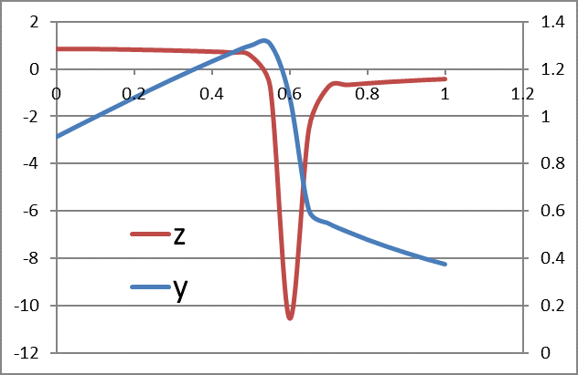
We solve the above stiff system for $ε = 0.01$ .

The solution steps are similar to Example 1. We work with the named variables, x, y, z, A, dA, eps corresponding to cells B2:B7 to define the system formulas and boundary condition matrix as shown in Table 1 below.

Table 1
	A	B	C	D
1		Variables	BCs
2	x		0	=y-0.9129
3	y	1	1	=y-0.375
4	z
5	A	=1+x^2
6	dA	=2*x
7	eps	0.01
8		Equations
9	dy/dx	=z
10	dz/dx	=((2.4/2-epsdA)yz-z/y-dA/A(1-0.4/2y^2))/(epsA*y)

Note that we assigned a non zero initial guess value for variable y to avoide the divide by zero error.

Next, we evaluate the array formula =BVSOLVE(B9:B10, B2:B4, C2:D3, {0,1}, , , {"ERROREST", True}) in an allocated array H4:J26. The solver now converges successfully and produces the following result (Table 2) which is plotted in Figure 1.

Table 2
	H	I	J
4	x	y	z
5	0	0.9129	0.835223
6	0.05	0.954646	0.834019
7	0.1	0.996237	0.828936
8	0.15	1.037468	0.819592
9	0.2	1.078129	0.806201
10	0.25	1.118026	0.789141
11	0.3	1.15699	0.7689
12	0.35	1.194872	0.745969
13	0.4	1.231542	0.72026
14	0.45	1.26676	0.684865
15	0.5	1.298649	0.549927
16	0.55	1.305552	-0.73972
17	0.6	1.083584	-10.5522
18	0.65	0.603002	-2.53229
19	0.7	0.547885	-0.76692
20	0.75	0.511759	-0.68353
21	0.8	0.479252	-0.6188
22	0.85	0.449708	-0.56442
23	0.9	0.422687	-0.51745
24	0.95	0.397869	-0.47612
25	1	0.375	-0.43931
26	Rel. Errors	8.33E-07	0.000237

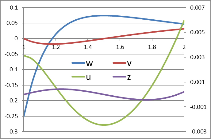
Example 3: Solving a fourth-order boundary value problem

This equation models a uniformly loaded beam of variable stiffness simply supported at both ends.

z^{''''} = \frac{1 - 6 x^{2} z^{'''} - 6 x z^{''}}{x^{3}}, 1 \leq x \leq 2

z (1) = 0, z^{''} (1) = 0, z (2) = 0, z^{''} (2) = 0

Using standard substitution technique we convert the 4th order equation to four 1st order equations.

Let $u = z', v = u^{'} = z^{''}, w = v^{'} = z''$

\frac{d w}{d x} = \frac{1 - 6 x^{2} w - 6 x v}{x^{3}}

\frac{d v}{d x} = w

\frac{d u}{d x} = v

\frac{d z}{d x} = u

The equivalent boundary conditions are $z (1) = 0, v (1) = 0, z (2) = 0, v (2) = 0$

Solution

The solution procedure is similar to Example 1 above. Working with the named variables x,u,v,w and z for cells B2:B6, we define the system equations and boundary conditions as shown in Table 1 below.

Table 1

	A	B	C	D
1	Variables		BCs
2	x		1	=z
3	u		1	=v
4	v		2	=z
5	w		2	=v
6	z
7	Equations
8	dw/dx	=(1-6x^2w-6xv)/x^3
9	dv/dx	=w
10	du/dx	=v
11	dz/dx	=u

To obtain the solution, We evaluate the array formula =BVSOLVE(B8:B11, B2:B6, C2:D5, {1,2}, , , {"ERROREST", True}) in allocated array H4:L26. The results are shown in Table 2 and plotted in Figure 1 below.

Table 2
	H	I	J	K	L
4	x	w	v	u	z
5	1	-0.5	1.55242E-30	0.017132	0
6	1.05	-0.33011	-0.02051609	0.016584	0.000847162
7	1.1	-0.20832	-0.03380919	0.0152	0.001644528
8	1.15	-0.12078	-0.04191665	0.013289	0.002358447
9	1.2	-0.05787	-0.04629629	0.011071	0.002968346
10	1.25	-0.0128	-0.048	0.008704	0.003463059
11	1.3	0.019257	-0.04779245	0.006302	0.003838168
12	1.35	0.041773	-0.04623279	0.003947	0.004094076
13	1.4	0.057268	-0.04373178	0.001695	0.004234597
14	1.45	0.067583	-0.04059207	-0.00042	0.004265921
15	1.5	0.074074	-0.03703704	-0.00236	0.004195851
16	1.55	0.077746	-0.03323151	-0.00412	0.00403324
17	1.6	0.079346	-0.02929688	-0.00568	0.003787576
18	1.65	0.079432	-0.02532209	-0.00704	0.003468679
19	1.7	0.078423	-0.02137187	-0.00821	0.003086471
20	1.75	0.076635	-0.01749271	-0.00918	0.002650819
21	1.8	0.074303	-0.01371742	-0.00996	0.002171412
22	1.85	0.071605	-0.01006851	-0.01056	0.001657686
23	1.9	0.068677	-0.00656072	-0.01097	0.00111876
24	1.95	0.065617	-0.00320302	-0.01121	0.0005634
25	2	0.0625	1.73472E-18	-0.01129	-1.0842E-19
26	Rel. Errors	3.17E-07	4.16988E-08	5.59E-09	8.15553E-10

Interior boundary conditions

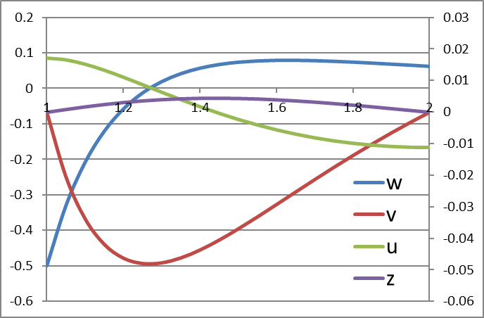
We can easily study the effect of the beam support locations. We solve the same problem but with the beam supported at left end and center (x=1 and x=1.5) with the right end free. The only required change to the problem setup is to change the values of the boundary points in cells C4 and C5 in Tabe 1 from 2 to 1.5. We re-run the solver and obtain the new solution plotted below.

Example 4: Solving a differential-algebraic (DAE) boundary value problem

Consider the following differential algebraic (DAE) system of equations

\frac{d u_{1}}{d x} = (ε + u_{2} - s i n (x)) y + c o s (x)

\frac{d u_{2}}{d x} = c o s (x)

\frac{d u_{3}}{d x} = y

0 = (u_{1} - s i n (x)) * (y - e^{x})

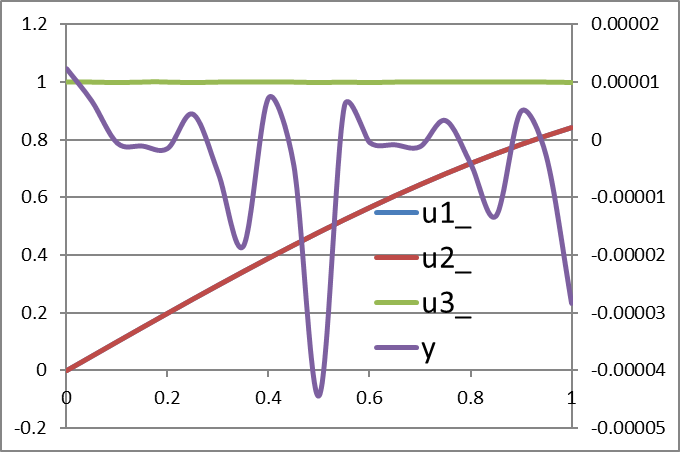
With boundary conditions

u_{1} (0) = s i n (0), u_{2} (1) = s i n (1), u_{3} (0) = 1, 0 \leq x \leq 1

For small values of $ε$ , this problem has the following solution

u_{1} = u_{2} = s i n (x); u_{3} = 1; y = 0

(See Ascher and Spiteri. Collocation software for boundary value differential-algebraic equations. SIAM Journal on Scientific Computing. Volume 15 938-952. 1995)

Solution

Working with the named variables x, u1_, u2_, u3_, y and eps for cells B2:B7, we define the system equations and boundary conditions as shown in Table 1 below.

Table 1
	A	B	C	D
1	Variables		BCs
2	x		0	=u1_-SIN(0)
3	u1_		0	=u3_-1
4	u2_		1	=u2_-SIN(1)
5	u3_
6	y
7	eps	0.001
8	Equations
9	du1/dx	=(eps+u2_-SIN(x))*y+COS(x)
10	du2/dx	=COS(x)
11	du3/dx	=y
12	0	=(u1_-SIN(x))*(y-EXP(x))

To obtain the solution, We evaluate the array formula =BVSOLVE(B9:B12, B2:B6, C2:D4, {0,1}, 1) in allocated array H4:L26 and obtain the results shown in Table 2 below.

Note that We used optional argument 5 to tell BVSOLVE that the last equation in B9:B12 is an algebraic equation.

Table 2
	H	I	J	K	L
4	x	u1_	u2_	u3_	y
5	0	0	0	1	1.238E-05
6	0.05	0.049979	0.049979	1	6.752E-06
7	0.1	0.099833	0.099833	1	-4.951E-07
8	0.15	0.149438	0.149438	1	-1.035E-06
9	0.2	0.198669	0.198669	1	-1.459E-06
10	0.25	0.247404	0.247404	1	4.503E-06
11	0.3	0.29552	0.29552	1	-5.653E-06
12	0.35	0.342898	0.342898	1	-1.840E-05
13	0.4	0.389418	0.389418	1	7.336E-06
14	0.45	0.434966	0.434966	1	-4.392E-06
15	0.5	0.479426	0.479426	1	-4.436E-05
16	0.55	0.522687	0.522687	1	5.825E-06
17	0.6	0.564642	0.564642	1	-4.189E-07
18	0.65	0.605186	0.605186	1	-8.164E-07
19	0.7	0.644218	0.644218	1	-1.141E-06
20	0.75	0.681639	0.681639	1	3.401E-06
21	0.8	0.717356	0.717356	1	-4.072E-06
22	0.85	0.75128	0.75128	1	-1.321E-05
23	0.9	0.783327	0.783327	1	4.991E-06
24	0.95	0.813416	0.813416	1	-2.817E-06
25	1	0.841471	0.841471	1	-2.832E-05

Algorithms

BVSOLVE is based on the COLDAE collocation method with adaptive mesh refinement.

References

U. Ascher and R. Spiteri. Collocation software for boundary value differential-algebraic equations, SIAM Journal on Scientific Computing. 15,938-952, (1994).
Ascher U M, Mattheij R M M and Russell R D. Numerical Solution of Boundary Value Problems for Ordinary Differential Equations, Prentice Hall, (1988).

ExcelWorks LLC

Solving boundary value problems in Excel

Syntax

=BVSOLVE(eqns, vars, bcs, domain, [options])

Boundary Conditions

Required Inputs

Optional Inputs

Solution

Solution

Solution

Interior boundary conditions

Solution

`=BVSOLVE(eqns, vars, bcs, domain, [options])`