
=IVSOLVE(eqns, vars, domain, [options])
Use IVSOLVE to solve an initial-value ordinary (ODE) or differential-algebraic (DAE) equation system stated in either of the canonical
forms below: (the system can have as many equations as needed.)
Example: With optional one or more algebraic equations:
Example:
To complete description of the problem, initial values for the variables yi are required.
eqns a reference to the system formulas (f1, f2,..,g1,..).
For a DAE system, algebraic equations must be listed after differential equations.
vars a reference to the system variables in the following order (t, y1, y2,.. ). Each state variable must be assigned an initial value.
For a DAE system, algebraic variables should be orderd last in vars.
Variables order must be consistent with equations order. For example, given this order (t, y1, y2,.. ) implies dy1/dt = f1, dy2/dt = f2 and so forth.
Enter as a reference to a range. for Example, X1:X3. If your variables are not in a
contiguous range, say T1, X1, Y1, you can combine them and pass them as one reference as follows:
Use range union syntax (T1, X1:Y1) . Supported in ExceLab 7 only
Use array constant syntax {T1, X1, Y1}. Supported in Google Sheets only
ExceLab 365 supports only contiguous range input for multiple variables but, for convenience, will accept passing noncontiguous variables as string value "(T1,X1,Y1)"
domain a vector defining the start and end values for the time interval as well as the desired solution output time values.
| Format | Remarks |
|---|---|
| {ti, tf} | The interval [ti, tf] is divided uniformly according to the number of allocated rowsin the output array. |
| {{ti, tf, ndiv} | The interval [ti, tf] is divided uniformly into ndiv subintervals.The allocated output array must have sufficient rows to hold the result. |
| {ti, t1, t2, .., tf} | Solution results are reported for the supplied values only. The allocated output array must have sufficient rows to hold the result. |
m the number of algebraic constraints for an explicit DAE system, or the full mass matrix for an implicit system.
tol controls the absolute and relative error tolerances. Default values are 1.0e-4 for relative tolerance and 1.0e-6 for absolute tolerance.
Various formats are permitted as described below.
| Format | Remarks |
|---|---|
| rtol | Relative tolerance. Absolute tolerance value is set to rtol/100. Fixed for all variables. |
| {rtol, atol} | Relative and absolute tolerance values. Fixed for all variables |
| vector of rtoli | custom relative tolerance for each system variable. Absolute tolerance is set to rtoli/100. |
| two-column array of {rtoli, atoli} | custom relative and absolute tolerances for each system variable. |
ctrl a set of key/value pairs for algorithmic control as detailed below.
Description of key/value pairs for algorithmic control
| Key | ALGOR |
| Admissible Values (String) | RADAU5, BDF, ADAMS |
| Default Value | RADAU5 |
| Remarks | See Algorithms Section for details. |
| Key | MAXSTEPS |
| Default Value | 100000 (Integer) |
| Remarks | Sets an upper bound on the maximum number of integration steps that can be carried out. |
| Key | INITSTEP |
| Default Value | 1.0e-5 (Real) |
| Remarks | The step size is quickly adapted. A small value is recommended if the system has fast initial transients. |
| Key | STEPLIMIT |
| Default Value | Unbounded (Real) |
| Remarks | By setting a limit, accuracy may be improved at the expense of speed. |
| Key | JACSTEP |
| Admissible Values (Real) | 0 < JACSTEP < 0.1 |
| Default Value | The default step is computed dynamically based on machine accuracy, preset limits and function metric. For an order(1) function it is approximately 1.0e-8. |
| Remarks | The default value generally produces accurate approximations; however relaxing the default value may aid convergence on some problems with unknown Jacobian such as parameterized problems. |
| Key | JACSCHEME |
| Admissible Values (Integer) | 1 for First order Euler forward scheme 2 for Second order Euler forward scheme |
| Default Value | 1 |
| Remarks | First order scheme is generally sufficient. |
IVSOLVE is evaluated as an array formula in an allocated range of the spreadsheet. It computes and displays a formatted solution as illustrated in Figure 1 for a system with two state variables and a time domain [0 ,1]. The first column displays the time points, and the subsequent columns display the corresponding values of the state variables.
| A | B | C | |
| 1 | t | y1 | y2 |
| 2 | 0 | y1(0) | y2(0) |
| 3 | 0.1 | ↓ | ↓ |
| 4 | 0.2 | ||
| .. | ↓ | ||
| 12 | 1 | y1(1) | y1(1) |
When allocating a range for BVSOLVE, the following rules apply:
The number of allocated columns should match the number of variables.
The number of allocated rows is arbitrary. It determines the increment for the time interval subdivisions (only for display purpose).
You can customize the output time points using any of the following formats in argument number 3.
| Format | Remarks |
|---|---|
| {ti, tf} | The interval [ti, tf] is divided uniformly according to the number of allocated rowsin the output array. |
| {{ti, tf, ndiv} | The interval [ti, tf] is divided uniformly into ndiv subintervals.The allocated output array must have sufficient rows to hold the result. |
| {ti, t1, t2, .., tf} | Solution results are reported for the supplied values only. The allocated output array must have sufficient rows to hold the result. |
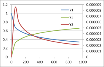
The following rate equations describe a chemical reaction
This system time domain is [0,1000] with initial conditions y1 = 1, y2 = y3 = 0
We pick T1 to represent the time variable and Y1, Y2, Y3 to represent the differential (state) variables, and define the system right-hand-side formulas in terms of our selected variables in range A1:A3 as shown in Table 1. We also assign the initial conditions for the state variables as shown in Table 1.
| A | Y | |
| 1 | =-0.04*Y1+10000*Y2*Y3 | 1 |
| 2 | =0.04*Y1-10000*Y2*Y3-30000000*Y2^2 | 0 |
| 3 | =30000000*Y2^2 | 0 |
Next, we evaluate the array formula =IVSOLVE(A1:A3, (T1,Y1:Y3), {0,1000}) in range
G4:J25 to obtain the solution shown in Table 2.
The first argument to IVSOLVE is the reference to the system RHS formulas defined in A1:A3. The second parameter is the reference
to the selected system variables. Note that we have used Excel union operator, (), to combine the time variable T1 and the state variables Y1:Y3 into one reference.
The third parameter is the time domain for the problem which is passed using Excel constant array syntax, {}, for convenience. Since we have used default format for output, IVSOLVE
reports the solution at a uniform time subdivision of the interval [0,1000] based on the number of allocated rows in the allocated range for output. You can control the output by allocating
a larger range or using other optional formats for parameter 3 to control the subdivison or the exact outputed time points.
Note. Passing the non contiguous variables as (T1,Y1:Y3) is supported in ExceLab 7 only. ExceLab 365 users pass as "(T1,Y1:Y3)". Google Sheets users pass as {T1,Y1:Y3}
| G | H | I | J | |
| 4 | T1 | Y1 | Y2 | Y3 |
| 5 | 0 | 1 | 0 | 0 |
| 6 | 50 | 0.693298 | 8.34608E-06 | 0.307238 |
| 7 | 100 | 0.617624 | 6.15491E-06 | 0.382913 |
| 8 | 150 | 0.570603 | 5.12544E-06 | 0.429936 |
| 9 | 200 | 0.5362 | 4.48885E-06 | 0.464339 |
| 10 | 250 | 0.509024 | 4.04263E-06 | 0.491515 |
| 11 | 300 | 0.486573 | 3.70661E-06 | 0.513967 |
| 12 | 350 | 0.467464 | 3.44094E-06 | 0.533076 |
| 13 | 400 | 0.450831 | 3.22379E-06 | 0.549709 |
| 14 | 450 | 0.436131 | 3.04165E-06 | 0.56441 |
| 15 | 500 | 0.422975 | 2.88612E-06 | 0.577566 |
| 16 | 550 | 0.411062 | 2.75081E-06 | 0.589479 |
| 17 | 600 | 0.400208 | 2.63192E-06 | 0.600333 |
| 18 | 650 | 0.390244 | 2.52635E-06 | 0.610297 |
| 19 | 700 | 0.381027 | 2.43154E-06 | 0.619514 |
| 20 | 750 | 0.372468 | 2.34583E-06 | 0.628073 |
| 21 | 800 | 0.364491 | 2.26794E-06 | 0.63605 |
| 22 | 850 | 0.357023 | 2.19669E-06 | 0.643519 |
| 23 | 900 | 0.35 | 2.13113E-06 | 0.650541 |
| 24 | 950 | 0.343382 | 2.07052E-06 | 0.65716 |
| 25 | 1000 | 0.337127 | 2.01432E-06 | 0.663415 |
This is a variation of Example 1 where y3 is treated as an algebraic variable. This system time domain is [0,1000] with initial conditions y1 = 1, y2 = y3 = 0
The solution steps are similar to Example 1. The RHS formulas are defined in A4:A6 as shown in Table 1 in terms of the selected variables T1 and Y1, Y2, Y3. Note that Y3 represents now an algebraic variable rather than a differential variable.
| A | |
| 4 | =-0.04*Y1+10000*Y2*Y3 |
| 5 | =0.04*Y1-10000*Y2*Y3-30000000*Y2^2 |
| 6 | =Y1+Y2+Y3-1 |
Next, we evaluate the array formula =IVSOLVE(A4:A6, (T1,Y1:Y3), {0,1000}, 1) in an allocated
range to obtain the solution.
Note that we pass 1 in the 4rth parameter to tell
the IVSOLVE that we have one algebraic equation in the system. Algebraic equations and variables must be ordered last. Here the solver will treat the last formula
as an algebraic equation along with variable Y3.
Note. Passing the non contiguous variables as (T1,Y1:Y3) is supported in ExceLab 7 only. ExceLab 365 users pass as "(T1,Y1:Y3)". Google Sheets users pass as {T1,Y1:Y3}
The new results, are only slightly different from Example 1, however, we extract below a sample to show that the solution satisfies the algebraic constraint Y1+Y2+Y3-1=0 as shown in Table 2.
| Y1 | Y2 | Y3 | Value of Y1+Y2+Y3-1 |
| 1 | 0 | 0 | 0 |
| 0.692879 | 8.34419E-06 | 0.307113 | -3.1E-13 |
| 0.617245 | 6.15373E-06 | 0.382749 | 3.31E-13 |
| 0.570232 | 5.12416E-06 | 0.429763 | -2.1E-13 |
| 0.535846 | 4.48774E-06 | 0.464149 | 7.77E-14 |
| 0.508695 | 4.04186E-06 | 0.491301 | 0 |
Next, we demonstrate how to use additional optional arguments.
We define the system Jacobian in M3:O5 and custom tolerances for variables Y1, Y2 and Y3 in the vector Q3:Q5 as shown in Table 3. We name these two ranges in Excel as jacob and rtol respectively.
| M | N | O | Q | ||
| 3 | -0.04 | =10000*Y3 | =10000*Y2 | 0.00001 | |
| 4 | 0.04 | =-10000*Y3-30000000*2*Y2 | =-10000*Y2 | 0.0000001 | |
| 5 | 1 | 1 | 1 | 0 |
We evaluate the updated array formula =IVSOLVE(A4:A6, (T1,Y1:Y3), {0,1000,16}, 1, rtol, jacob) in an allocated array M7:P25 and obtain the new solution shown in Table 4.
Notice that we requested in argument 3 to use exactly 16 subdivisions for the output time interval. This fills rows 8 through 24. Any extra
rows in the allocated array are filled with zeros.
| M | N | O | P | |
| 7 | T1 | Y1 | Y2 | Y3 |
| 8 | 0 | 1 | 0 | 0 |
| 9 | 62.5 | 0.669227 | 7.57291E-06 | 0.330766 |
| 10 | 125 | 0.591594 | 5.56659E-06 | 0.408401 |
| 11 | 187.5 | 0.54362 | 4.62411E-06 | 0.456375 |
| 12 | 250 | 0.508685 | 4.04171E-06 | 0.491311 |
| 13 | 312.5 | 0.481197 | 3.63374E-06 | 0.518799 |
| 14 | 375 | 0.45856 | 3.3264E-06 | 0.541437 |
| 15 | 437.5 | 0.439342 | 3.08361E-06 | 0.560655 |
| 16 | 500 | 0.422672 | 2.88522E-06 | 0.577325 |
| 17 | 562.5 | 0.407969 | 2.71896E-06 | 0.592028 |
| 18 | 625 | 0.394837 | 2.57688E-06 | 0.60516 |
| 19 | 687.5 | 0.382986 | 2.45358E-06 | 0.617012 |
| 20 | 750 | 0.372201 | 2.3452E-06 | 0.627796 |
| 21 | 812.5 | 0.362313 | 2.24888E-06 | 0.637685 |
| 22 | 875 | 0.353197 | 2.16257E-06 | 0.646801 |
| 23 | 937.5 | 0.344745 | 2.08461E-06 | 0.655253 |
| 24 | 1000 | 0.336875 | 2.01371E-06 | 0.663122 |
| 25 | 0 | 0 | 0 | 0 |
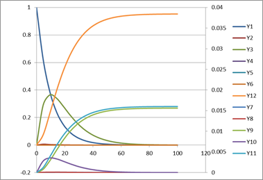
The following system with 12 rate equations arises from chemical kinetics.
We solve this system in the time interval [0,100] starting from initial conditions: y1 = 1 and 0 for the rest.
The steps to solve this system are similar to Example 1. We define the RHS system formulas in A26:A37 using variables T1, and Y1:Y12 as shown in Table 1. Variable Y1 is assigned the value 1 for the initial condition whereas the remaining variables Y2:Y12 are left blank consistent with the initial condition of 0.
| A | |
| 26 | =-0.1*Y1 |
| 27 | =0.1*Y1+1500*Y4+1500*Y5-50*Y2*Y3-100*Y2*Y12-10*Y2 |
| 28 | =10*Y2-0.1*Y3-50*Y2*Y3-50*Y10*Y3+1500*Y4+1500*Y6 |
| 29 | =50*Y2*Y3-1502.5*Y4 |
| 30 | =100*Y2*Y12-1502.5*Y5 |
| 31 | =50*Y10*Y3-1502.5*Y6 |
| 32 | =100*Y10*Y12-1502.5*Y7 |
| 33 | =50*Y10-1505*Y8 |
| 34 | =2.5*Y4+2.5*Y5+2.5*Y6+2.5*Y7 |
| 35 | =0.1*Y3+1500*Y6+1500*Y7+1500*Y8-50*Y10*Y3-100*Y10*Y12-10*Y10-50*Y10 |
| 36 | =5*Y8 |
| 37 | =10*Y10+1500*Y5+1500*Y7-100*Y2*Y12-100*Y10*Y12 |
To obtain the solution, we evaluate the array formula =IVSOLVE(A26:A37, (T1,Y1:Y12), {0,100}) in allocated array J4:V26. The results are plotted in the figure below.
Note. Passing the non contiguous variables as (T1,Y1:Y12) is supported in ExceLab 7 only. ExceLab 365 users pass as "(T1,Y1:Y12)". Google Sheets users pass as {T1,Y1:Y12}
IVSOLVE offers the following algorithms: