
=PDASOLVE(eqns, vars, bcs, xdom, tdom, [options])
Note. PDASOLVE is available in ExceLab 7 only. Will be enabled in ExceLab 365 and Google Sheets in a future release.
PDASOLVE is a versatile solver for partial differential equations that supports advanced modeling capabilities including:
Use
PDASOLVE to solve a system of partial differential equations the following forms:
(the system can have as many equations as needed)
where , ,
Initial value for each variable ui is required.
PDASOLVE supports general boundary conditions that can be specified at arbitrary locations within the system's spatial domain.
The boundary condition types are described below:
eqns a reference to the system formulas (f1, f2,.., g1,..).
For a DAE system, algebraic equations must be listed after differential equations.
vars a reference to the system variables in the following order (
t, x, u1, u2,.. ,
u1,x, u2,x,..,
u1,xx, u2,xx,..
). The state variables (u1, u2,..)
must be assigned initial conditions. An initial condition can be a constant or function of the spatial variable x.
All the variables and derivatives must be defined in the order listed above in
vars regardless if they are used in the equations or not.
For a DAE system, algebraic variables should be orderd last in vars.
bcs A reference to a 3-column matrix defining the system's boundary conditions.
The first column specifies the x locations of the boundary conditions,
the 2nd column specifies the types which can by any of the letters 'D', 'N', 'R' or 'C',
and the 3rd column specifies the boundary condition formulas.
A boundary condition formula is arranged with respect to zero on one side.
Example of a boundary conditions matrix
| E | F | G | |
| 10 | 0 | D | =U1-1 |
| 11 | 1 | R | =UX1-0.5*U1-2 |
| 12 | 0.5 | C | =K1*UX1 |
xdom a vector defining the start and end values for the spatial domain as well as the desired solution output spatial values.
If an equation is defined only over a sub region of the spatial domain, also use argument 7 to define custom regions.
| Format | Remarks |
|---|---|
| {xs, xe} | The domain [xs, xe] is divided uniformly according to the allocated output array size. |
| {xs, xe, ndiv} | The domain [xs, xe] is divided uniformly into ndiv subintervals. |
| {xs, x1, x2, .., xe} | Solution results are reported for the supplied values only. |
tdom a vector defining the start and end values for the time interval as well as the desired solution output time values.
| Format | Remarks |
|---|---|
| {ti, tf} | The interval [ti, tf] is divided uniformly according to the allocated output array size. |
| {ti, tf, ndiv} | The interval [ti, tf] is divided uniformly intondiv subintervals. |
| {ti, t1, t2, .., tf} | Solution results are reported for the supplied values only. |
m the number of algebraic equations for an explicit DAE system, or the full mass Matrix for an implicit system.
rgns
A 2-column matrix defining the subdomain for each equation. Each row specifies the left and right region endpoints for the corresponding equation in eqns.
. By default, all equations in the system are assumed to share the entire spatial domain defined in argument 4.
tol controls the absolute and relative error tolerances for temporal integration algorithm.
Default values are 1.0e-4 for relative tolerance and 1.0e-6 for absolute tolerance. Various formats are permitted as described below.
| Format | Remarks |
|---|---|
| rtol | Relative tolerance. Absolute tolerance value is set to rtol/100. Fixed for all variables. |
| {rtol, atol} | Relative and absolute tolerance values. Fixed for all variables |
| vector of rtoli | custom relative tolerance for each system variable. Absolute tolerance is set to rtoli/100. |
| two-column array of {rtoli, atoli} | custom relative and absolute tolerances for each system variable. |
ctrl a set of key/value pairs for algorithmic control as detailed below.
Description of key/value pairs for algorithmic control
| Key | NDRVOUT |
| Admissible Values (Integer) |
|
| Default Value | 0 |
| Remarks | The allocated results array must have sufficient columns to hold output. |
| Key | FORMAT |
| Admissible Values (String) |
XCOL1 TCOL1 |
| Default Value | XCOL1 |
| Remarks | XCOL1 format is convenient to plot snapshots of solution variables at a desired time values. TCOL1 format is convenient to plot transient views of solution variables at a desired spatial locations. See Output Format section for more detail. |
| Key | MAXSTEPS |
| Default Value | 100000 (Integer) |
| Remarks | Sets an upper bound on the maximum number of integration steps that can be carried out. |
| Key | INITSTEP |
| Default Value | 1.0e-5 (Real) |
| Remarks | The step size is quickly adapted. A small value is recommended if the system has fast initial transients. |
| Key | STEPLIMIT |
| Default Value | Unbounded (Real) |
| Remarks | By setting a limit, accuracy may be improved at the expense of speed. |
| Key | MAX_GRID_SPACING |
| Default Value | 0.01 (Real) |
| Remarks | Sets a a limit on the maximum distance between adjacent grid nodes. All distances between adjacent grid nodes will be less than or equal toMAX_GRID_SPACING. This value has direct impact on computational cost. |
| Key | MIN_GRID_SPACING |
| Default Value | 0.000001 (Real) |
| Remarks | Sets a limit on the minimum distance between adjacent grid nodes. All distances between adjacent grid nodes will greater than or equal toMIN_GRID_SPACING. |
| Key | MAX_GRID_NODES |
| Default Value | 2000 (Integer) |
| Remarks | Sets a limit on the maximum allowed number of generated nodes in the system spatial domain. |
| Key | MIN_GRID_NODES |
| Default Value | 10 (Integer) |
| Remarks | Sets a limit on the minimum number of generated nodes in any subregion of the system spatial domain. |
| Key | JACSTEP |
| Admissible Values (Real) | 0 < JACSTEP < 0.1 |
| Default Value | The default step is computed dynamically based on machine accuracy, preset limits and function metric. For an order(1) function it is approximately 1.0e-8. |
| Remarks | The default value generally produces accurate approximations; however relaxing the default value may aid convergence on some problems with unknown Jacobian such as parameterized problems. |
| key | JACSCHEME |
| Admissible Values (Integer) | 1 for First order Euler forward scheme 2 for Second order Euler forward scheme |
| Default Value | 1 |
| Remarks | First order scheme is generally sufficient. |
To illustrate PDASOLVE output layout, we consider a 2-equation system with the following variables
(t, x, u1, u2, u1,x, u2,x, u1,xx, u2,xx)
The snapshot view is the default format. It allows you to easily plot snapshot views for the variables at desired time points. In this format, the solution is laid out as shown in Table 1. Output spatial points are listed in the first column starting at row 3, whereas output time points are listed in blocks in the first row starting at column 2 with variables names listed in the second row.
| A | B | C | D | E | F | G | H | .. | |
| 1 | t → | t0 | t0 | t1 | t1 | t2 | t2 | .. | tf |
| 2 | x ↓ | u1 | u2 | u1 | u2 | u1 | u2 | .. | u2 |
| 3 | xs | ||||||||
| 4 | x1 | u2(x1,t0) | |||||||
| 5 | x2 | ||||||||
| .. | .. | ||||||||
| N | xe |
The spatial and time domain are divided uniformly according to the number of allocated rows and columns for the output array.
You can control x and t values by specifying your own step or custom values in parameters 4 and 5
for PDASOLVE.
If you allocate a larger array than needed, unused rows and columns will be filled with zeros.
You can find out the minimum array size needed by evaluating PDASOLVE formula initially in one cell.
We can request to report 1st and 2nd derivative variables using the key NDRVOUT with value 1 or 2. Table 2 shows the modified layout with NDRVOUT value set to 1, in which values for u1,x, and u2,x are also included.
| A | B | C | D | E | F | G | H | I | J | .. | |
| 1 | t → | t0 | t0 | t0 | t0 | t1 | t1 | t1 | t1 | .. | tf |
| 2 | x ↓ | u1 | u2 | u1,x | u2,x | u1 | u2 | u1,x | u2,x | .. | u2,x |
| 3 | xs | ||||||||||
| 4 | x1 | ||||||||||
| 5 | x2 | u1(x2,t1) | |||||||||
| .. | .. | ||||||||||
| N | xe |
In this format, the roles of x and t are interchanged. Output time points are displayed in the first column, whereas spatial points are displayed in the first row. This format allows you to easily plot transient views of the variables at desired spatial points.
This example is discussed in detail in the following publication:
Ghaddar C.K., Rapid Modeling and Parameter Estimation of Partial Differential Algebraic Equations by a Functional Spreadsheet Paradigm.Math. Comput. Appl. 2018, 23, 39.
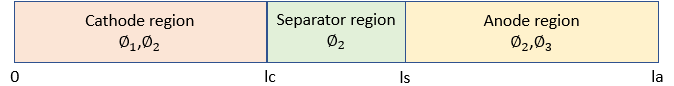
Where
| x = 0 | x = lc | x = ls | x = la |
|---|---|---|---|
Working with named system variables, parameters, and property functions, we define the complete Excel model including equations, regions, and boundary conditions formulas as shown in Table 1.
| A | B | C | D | E | F | G | H | |
| 1 | System Variables with initial values | System Parameters | ||||||
|---|---|---|---|---|---|---|---|---|
| 2 | t | lc | 2.00E-04 | |||||
| 3 | x | ls | 2.254E-04 | |||||
| 4 | phi_1 | 0 | la | 4.254E-04 | ||||
| 5 | phi_2 | 0 | beta | 1 | ||||
| 6 | phi_3 | 0 | gamma | 0.5 | ||||
| 7 | phi1x | mc | 1E+06 | |||||
| 8 | phi2x | |||||||
| 9 | phi3x | Mass Matrix | ||||||
| 10 | phi1xx | 1E+06 | =-mc | 0 | ||||
| 11 | phi2xx | =-mc | 1E+06 | =-mc | ||||
| 12 | phi3xx | 0 | =-mc | 1E+06 | ||||
| 13 | ||||||||
| 14 | Property Functions | x Domain | 0 | =la | ||||
| 15 | sigma | =IF(x<=lc,1,IF(x<ls,0,1)) | t Interval | 0 | 1 | Boundary conditions matrix | ||
| 16 | kappa | =beta*IF(x<=lc,1,IF(x<ls,2,1)) | 0 | R | =sigma*phi1x-1 | |||
| 17 | a | =gamma*IF(x<=lc,1E6,IF(x<ls,0,1E6)) | 0 | N | =phi2x | |||
| 18 | f | =IF(x<=lc,3*EXP(-2*t),0) | =lc | N | =phi1x | |||
| 19 | =lc | C | =kappa*phi2x | |||||
| 20 | System RHS Equations | Regions | =ls | C | =kappa*phi2x | |||
| 21 | eq1 | =sigma*phi1xx-a*(phi_1-phi_2-f) | 0 | =lc | =ls | N | =phi3x | |
| 22 | eq2 | =kappa*phi2xx+a*(phi_1-phi_2-f) | 0 | =la | =la | N | =phi2x | |
| 23 | eq3 | =sigma*phi3xx-a*(phi_3-phi_2-f) | =ls | =la | =la | D | =phi_3 | |
To aid readability, we assign assign names for selected Excel ranges in Table 1 which represent input arguments to PDASOLVE as shown in Table 2.
| Excel Range | Assigned Name |
|---|---|
| B21:B23 | Eqns |
| B2:B12 | Vars |
| F16:H23 | BCs |
| D14:E14 | xDom |
| D15:E15 | tDom |
| C10:E12 | M |
| C21:D23 | Rgns |
Next, we evaluate the formula
=PDASOLVE(Eqns, Vars, BCs, xDom, tDom, M, Rgns, , {"FORMAT","TCOL1"})
in array G15:S27 and obtain the solution as shown in Table 3.
| G | H | I | J | K | L | M | N | O | P | Q | R | S | |
| 15 | x | 0 | 0 | 0 | 0.0002 | 0.0002 | 0.0002 | 0 | 0.0002254 | 0.0002254 | 0.0004254 | 0.0004254 | 0.00043 |
| 16 | t | phi_1 | phi_2 | phi_3 | phi_1 | phi_2 | phi_3 | phi_1 | phi_2 | phi_3 | phi_1 | phi_2 | phi_3 |
| 17 | 0 | 0 | 0 | 0 | 0 | 0 | 0 | 0 | 0 | 0 | 0 | 0 | 0 |
| 18 | 0.1 | 0.0490406 | -0.0031269 | 0 | 0.0491381 | -0.0026646 | 0 | 0 | -0.0026093 | -0.0003937 | 0 | -0.002235 | 0 |
| 19 | 0.2 | 0.0888748 | -0.004782 | 0 | 0.0889728 | -0.0043945 | 0 | 0 | -0.0043481 | -0.0003311 | 0 | -0.004033 | 0 |
| 20 | 0.3 | 0.1204078 | -0.0061393 | 0 | 0.1205061 | -0.0058129 | 0 | 0 | -0.0057737 | -0.0002801 | 0 | -0.005507 | 0 |
| 21 | 0.4 | 0.1451792 | -0.0072539 | 0 | 0.1452778 | -0.0069774 | 0 | 0 | -0.0069442 | -0.0002385 | 0 | -0.006716 | 0 |
| 22 | 0.5 | 0.1644121 | -0.0081697 | 0 | 0.164511 | -0.0079339 | 0 | 0 | -0.0079055 | -0.0002046 | 0 | -0.00771 | 0 |
| 23 | 0.6 | 0.1791579 | -0.0089244 | 0 | 0.179257 | -0.0087217 | 0 | 0 | -0.0086973 | -0.0001769 | 0 | -0.008528 | 0 |
| 24 | 0.7 | 0.1902228 | -0.0095468 | 0 | 0.190322 | -0.0093711 | 0 | 0 | -0.0093499 | -0.0001544 | 0 | -0.009201 | 0 |
| 25 | 0.8 | 0.1983065 | -0.0100621 | 0 | 0.1984059 | -0.0099083 | 0 | 0 | -0.0098896 | -0.0001361 | 0 | -0.009758 | 0 |
| 26 | 0.9 | 0.2039649 | -0.01049 | 0 | 0.2040644 | -0.010354 | 0 | 0 | -0.0103374 | -0.0001213 | 0 | -0.01022 | 0 |
| 27 | 1 | 0.2076535 | -0.0108468 | 0 | 0.2077531 | -0.0107253 | 0 | 0 | -0.0107105 | -0.0001093 | 0 | -0.010605 | 0 |
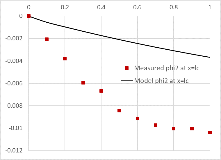
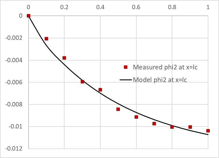
In Figure 1, we plot phi2(x,t) at the interface x = lc together with imperical values for Φ(lc,t) Clearly the default model does not agree well with experimental data. In Example 2, we will show you how to optimize the model parameters so it agrees with experimental data accurately.
The result shown in Table 1, is insufficient to verify the flux continuity conditions and are staisfied at the regions interfaces x = lc and x = ls. Here, we illustrate use of additional optional parameters to report the 1st derivatives at custom spatial points just before and after x = lc and x = ls, as well as, enhance the solution accuracy.
Table 4 shows the definition of new optional parameters consisting of: custom output points in G20:N20 which is named as xOut; relative tolerances in D21:D23 which is named as rTols; and a set of key/value pairs in A21:B23 which is named Cntrls. The keys include NDRVOUT with a value of 1, to report the first derivative in the output, and MAX_GRID_SPACING which ensures that the maximum distance between computational spatial grid nodes does not exceed the specified value of 1.0e-5.
| A | B | C | D | E | F | G | H | I | J | K | L | M | N | |
| 20 | Solver Options | Rel. Tolerance | xout | 0 | =lc-0.001*lc | =lc | =lc+0.001*lc | =ls-0.001*ls | =ls | =ls+0.001*ls | =la | |||
|---|---|---|---|---|---|---|---|---|---|---|---|---|---|---|
| 21 | FORMAT | TCOL1 | 0.0001 | |||||||||||
| 22 | NDRVOUT | 1 | 0.000001 | |||||||||||
| 23 | MAX_GRID_SPACING | 0.00001 | 0.000001 |
We evaluate the enhanced formula
=PDASOLVE(Eqns, Vars, BCs, xOut, tDom, M, Rgns, rTols, Cntrls)
in array A50:AW62 to obtain a new solution. We show in Table 5 values for phi2x just before and after
the interfaces at x = lc and x = ls. A quick inspection of the ratios
, and
in Table 5 shows that the flux continuity conditions are satisfied at all times
| L | R | X | AD | AJ | AP | |||
| 50 | x | 0.0001998 | 0.0002 | 0.0002002 | .. | 0.00022517 | 0.000225 | 0.000225625 |
| 51 | t | phi2X | phi2x | phi2x | phi2x | phi2x | phi2x | |
| 52 | 0 | 0 | Undef | 0 | 0 | Undef | 0 | |
| 53 | 0.1 | 0.999180576 | Undef | 0.49957693 | 0.44674817 | Undef | 0.891514551 | |
| 54 | 0.2 | 0.999180576 | Undef | 0.49959529 | 0.44905949 | Undef | 0.89617388 | |
| 55 | 0.3 | 0.999180577 | Undef | 0.49961286 | 0.45127134 | Undef | 0.900632825 | |
| 56 | 0.4 | 0.999180568 | Undef | 0.49962967 | 0.45338715 | Undef | 0.904898145 | |
| 57 | 0.5 | 0.999180579 | Undef | 0.49964575 | 0.45541108 | Undef | 0.908978265 | |
| 58 | 0.6 | 0.999180562 | Undef | 0.49966113 | 0.45734714 | Undef | 0.912881228 | |
| 59 | 0.7 | 0.999180583 | Undef | 0.49967585 | 0.45919913 | Undef | 0.916614717 | |
| 60 | 0.8 | 0.999180566 | Undef | 0.49968992 | 0.46097071 | Undef | 0.920186109 | |
| 61 | 0.9 | 0.999180582 | Undef | 0.49970339 | 0.46266537 | Undef | 0.92360242 | |
| 62 | 1 | 0.999180573 | Undef | 0.49971627 | 0.46428644 | Undef | 0.926870399 |
This example is a continuation of Example 1.
The computed values for phi2 at the interface x = lc based on the default system parameters, are clearly in disagreement with the observed data as shown in Figure 1 of Example 1. The observed values for Φ(lc,t) are give in Table 6.
| M | N | |
| 1 | time | Emperical phi2 |
|---|---|---|
| 2 | 0 | 0 |
| 3 | 0.1 | -0.002052705 |
| 4 | 0.2 | -0.00380538 |
| 5 | 0.3 | -0.005944579 |
| 6 | 0.4 | -0.006668727 |
| 7 | 0.5 | -0.008436437 |
| 8 | 0.6 | -0.009136398 |
| 9 | 0.7 | -0.009734491 |
| 10 | 0.8 | -0.010031262 |
| 11 | 0.9 | -0.010050529 |
| 12 | 1 | -0.010387955 |
Our task is to compute optimal values for the design parameters γ, and mc which minimize the sum of square residuals between our
model predictions and the observed data in Table 6. We have two options to solve this dynamical minimization problem: Excel built-in NLP Solver;
and NLSOLVE.
We demonstrate both procedures below.
We define an objective formula to be minimized. The objective formula calculates the summation of the square residuals between the observed values and their corresponding computed values from the solution result in Table 3 of Example 1. The definition of the objective formula is shown in S2 of Table 7 with initial value of 0.00033.
| P | S | |
| 1 | =(L18-N2)^2 | Objective |
|---|---|---|
| 2 | =(L19-N3)^2 | =SUM(P1:P10) |
| 3 | =(L20-N4)^2 | |
| 4 | =(L21-N5)^2 | |
| 5 | =(L22-N6)^2 | |
| 6 | =(L23-N7)^2 | |
| 7 | =(L24-N8)^2 | |
| 8 | =(L25-N9)^2 | |
| 9 | =(L26-N10)^2 | |
| 10 | =(L27-N11)^2 | |
| 10 | =(L28-N12)^2 |
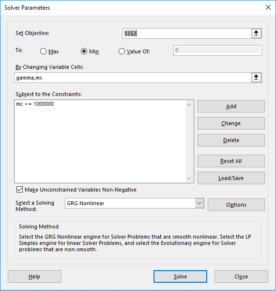
The remaining task is to configure and run Excel Solver command. We configure the solver exactly as shown in Figure 2. We select to minimize the objective formula S2, by varying gamma and mc, subject to the upper bound constraint mc <= 10e6 which is added for numerical stability since larger values for the off-diagonal mass matrix element mc leads to a divergent system.
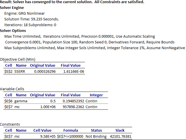
We run the solver which reports a feasible solution in less than a minute of computing time as shown in the Answer Report generated by the Excel Solver in Figure 3. Upon accepting the solution, Excel automatically updates the spreadsheet to reflect the optimal computed values. The optimized solution for phi2 is shown in Figure 4 exhibiting excellent agreement with observed values.
NLSOLVE
Unlike Excel Solver which requires an objective formula, NLSOLVE requires the list of individual residual constraint formulas which we define
as shown in Table 8.
| R | |
| 1 | =ARRAYVAL(L18)-N2 |
| 2 | =ARRAYVAL(L19)-N3 |
| 3 | =ARRAYVAL(L20)-N4 |
| 4 | =ARRAYVAL(L21)-N5 |
| 5 | =ARRAYVAL(L22)-N6 |
| 6 | =ARRAYVAL(L23)-N7 |
| 7 | =ARRAYVAL(L24)-N8 |
| 8 | =ARRAYVAL(L25)-N9 |
| 9 | =ARRAYVAL(L26)-N10 |
| 10 | =ARRAYVAL(L27)-N11 |
| 10 | =ARRAYVAL(L27)-N12 |
What is ARRAYVAL? ARRAYVAL is one of
the criterion functions that allow us to define dynamic constraints on the solution array for input to NLSOLVE.
In this case we are simply picking a value from the solution but in general, a criterion function can be used to specify more complex constraint on the solution.
Next, we evaluate the formula =NLSOLVE(R1:R10,(gamma,mc)) in array S4:T8 and obtain virtually the same solution found by Excel Solver
as shown in Table 9. However, NLSOLVE, converges in fewer iterations in less than one third of the time.
Since NLSOLVE is a pure spreadsheet function, it does not modify its arguments or update the spreadsheet calculation.
Therefore, to update the spreadsheet result, the computed values for gamma and mc must copied manually to
their respective variable cells D6 and D7 of Table 3 of Example 1.
| S | T | |
| 4 | gamma | 0.195638747 |
| 5 | mc | 958050.8287 |
| 6 | SSERROR | 1.61147E-06 |
| 7 | ITRN | 10 |
| 8 | TIME (s) | 18.729 |
PDASOLVE implements the method of lines. Spatial discretization is carried out using a second-order variable-step finite difference scheme,
and the resulting implicit DAE system is integrated by RADAU5 with adaptive step control.