Solving Partial Differential Equations in Excel

Syntax

`=PDSOLVE(eqns, vars, lbc, rbc, xdom, tdom, [options])`

Description

Use PDSOLVE to solve a system of partial differential equations the following form: (the system can have as many equations as needed)

\frac{\partial u_{1}}{\partial t} = f_{1} (t, x, u, u_{x}, u_{x x})

\frac{\partial u_{2}}{\partial t} = f_{2} (t, x, u, u_{x}, u_{x x})

where $u = [u_{1}, u_{2}]$ , $u_{x} = [u_{1, x}, u_{2, x}]$ , $u_{x x} = [u_{1, x x}, u_{2, x x}]$

Initial Conditions

Initial value for each variable u_i is required.

Boundary Conditions

General nonlinear boundary conditions can be specified at left and right ends of the system spatial domain [x_s,x_e].
Generally, for each equation f_i in the system: none, one or two boundary conditions are required depending on the order of the equation.

If f_i does not depend on $u_{i, x}$ and $u_{i, x x}$ then no boundary conditions are required for equation i.
If f_i depends only on $u_{i, x}$ then only one boundary condition is required for equation i.
If f_i depends depends on $u_{i, x x}$ then two boundary conditions are required for equation i.

Inputs

Required Inputs

eqns a reference to the system formulas (f₁, f₂,..).

vars a reference to the system variables in the following order ( t, x, u₁, u₂,.. , u_1,x, u_2,x,.., u_1,xx, u_2,xx,..). The state variables (u₁, u₂,..) must be assigned initial conditions. An initial condition can be a constant or function of the spatial variable x.

All the variables and derivatives must be defined in the order listed above in vars regardless if they are used in the equations or not.

Variables order must be consistent with equations order. For example, given this order (t, x, u₁, u₂,.. ) implies ∂u₁/∂t = f₁, ∂u₂/∂t = f₂ and so forth.

lbc a reference to the left boundary condition formulas for each equation in the system. Use the string "NA" to indicate an equation has no left boundary condition.

The number of left boundary conditions must equal the number of equations in eqns. Use the string "NA" to indicate an equation has no left boundary condition.

A boundary condition formula is arranged with respect to zero on one side. For Example, suppose that the boundary condition (BC) is u₁= u₂+1, then the BC formula may be defined as =U1-U2-1.

rbc a reference to the right boundary condition formulas for each equation in the system.

The number of right boundary conditions must equal the number of equations in eqns. Use the string "NA" to indicate an equation has no right boundary condition.

xdom a vector defining the start and end values for the spatial domain as well as the desired solution output spatial values.

Domain formats for solution spatial output control

Format	Remarks
{`x_s, x_e`}	The domain [`x_s, x_e`] is divided uniformly according to the allocated output array size.
{`x_s, x_e, ndiv`}	The domain [`x_s, x_e`] is divided uniformly into `ndiv` subintervals.
{`x_s, x₁, x₂, .., x_e`}	Solution results are reported for the supplied values only.

tdom a vector defining the start and end values for the time interval as well as the desired solution output time values.

Domain formats for solution temporal output control

Format	Remarks
{`t_i, t_f`}	The interval [`t_i, t_f`] is divided uniformly according to the allocated output array size.
{`t_i, t_f, ndiv`}	The interval [`t_i, t_f`] is divided uniformly into `ndiv` subintervals.
{`t_i, t₁, t₂, .., t_f`}	Solution results are reported for the supplied values only.

Optional Inputs

tol controls the absolute and relative error tolerances for temporal integration algorithm. Default values are 1.0e-4 for relative tolerance and 1.0e-6 for absolute tolerance. Various formats are permitted as described below.

Tolerance formats

Format	Remarks
`rtol`	Relative tolerance. Absolute tolerance value is set to `rtol/100`. Fixed for all variables.
{`rtol, atol`}	Relative and absolute tolerance values. Fixed for all variables
vector of `rtol_i`	custom relative tolerance for each system variable. Absolute tolerance is set to `rtol_i/100.`
two-column array of {`rtol_i, atol_i`}	custom relative and absolute tolerances for each system variable.

ctrl a set of key/value pairs for algorithmic control as detailed below.

Description of key/value pairs for algorithmic control

Solution Output and Format

Key	NDRVOUT
Admissible Values (Integer)	report only (`u₁, u₂,..`) in output. include first derivatives (`u_1,x, u_2,x,..`) in output. include first and second derivatives (`u_1,x, u_2,x,..`),(`u_1,xx, u_2,xx,..`) in output.
Default Value	0
Remarks	The allocated results array must have sufficient columns to hold output.

Key	FORMAT
Admissible Values (String)	XCOL1 Column 1 of the results array will contain the output spatial points.A block of columns for the solution variables at each output temporal point will be reported in order following column 1. TCOL1 Column 1 of the result array will contain the output temporal points.A block of columns for the solution variables at each output spatial point will be reported in order following column 1.
Default Value	XCOL1
Remarks	XCOL1 format is convenient to plot snapshots of solution variables at a desired time values. TCOL1 format is convenient to plot transient views of solution variables at a desired spatial locations. See Output Format section for more detail.

Algorithm Selection

Key	ALGOR
Admissible Values (String)	ADAMS, BDF, RADAU5
Default Value	BDF
Remarks	Use ADAMS for smooth problems, BDF or RADAU5 for stiff problems.

Temporal Integration Algorithm Parameters

Key	MAXORDBDF
Admissible Values (Integer)	2 ≤ MAXORDBDF ≤ 5
Default Value	5
Remarks	Maximum order for BDF. A higher value will increase computational cost.

Key	MAXORDADAMS
Admissible Values (Integer)	2 ≤ MAXORDADAMS ≤ 12
Default Value	12

Key	MAXSTEPS
Default Value	100000 (Integer)
Remarks	Sets an upper bound on the maximum number of integration steps that can be carried out.

Key	INITSTEP
Default Value	1.0e-5 (Real)
Remarks	The step size is quickly adapted. A small value is recommended if the system has fast initial transients.

Key	STEPLIMIT
Default Value	Unbounded (Real)
Remarks	By setting a limit, accuracy may be improved at the expense of speed.

Grid and Spatial Discretization

Key	NNODES
Default Value	50 (Integer)
Remarks	Number of mesh nodes for the spatial domain. This value has direct impact on computational cost.

Key	KORDER
Admissible Values (Integer)	2 ≤ KORDER ≤ 7
Default Value	4
Remarks	Number of collocation points per mesh subinterval. Higher values have direct impact on computational cost.

Jacobian Approximation

Key	JACSTEP
Admissible Values (Real)	`0 < JACSTEP < 0.1`
Default Value	The default step is computed dynamically based on machine accuracy, preset limits and function metric. For an order(1) function it is approximately 1.0e-8.
Remarks	The default value generally produces accurate approximations; however relaxing the default value may aid convergence on some problems with unknown Jacobian such as parameterized problems.

key	JACSCHEME
Admissible Values (Integer)	1 for First order Euler forward scheme 2 for Second order Euler forward scheme
Default Value	1
Remarks	First order scheme is generally sufficient.

Output Format

To illustrate PDSOLVE output layout, we consider a 2-equation system with the following variables (t, x, u₁, u₂, u_1,x, u_2,x, u_1,xx, u_2,xx)

Snapshot View Format

The snapshot view is the default format. It allows you to easily plot snapshot views for the variables at desired time points. In this format, the solution is laid out as shown in Table 1. Output spatial points are listed in the first column starting at row 3, whereas output time points are listed in blocks in the first row starting at column 2 with variables names listed in the second row.

Table 1
	A	B	C	D	E	F	G	H	..
1	`t` →	`t₀`	`t₀`	`t₁`	`t₁`	`t₂`	`t₂`	..	`t_f`
2	`x` ↓	`u₁`	`u₂`	`u₁`	`u₂`	`u₁`	`u₂`	..	`u₂`
3	`x_s`
4	`x₁`		`u₂(x₁,t₀)`
5	`x₂`
..	..
`N`	`x_e`

The spatial and time domain are divided uniformly according to the number of allocated rows and columns for the output array. You can control x and t values by specifying your own step or custom values in parameters 4 and 5 for PDSOLVE.
If you allocate a larger array than needed, unused rows and columns will be filled with zeros. You can find out the minimum array size needed by evaluating PDSOLVE formula initially in one cell.

We can request to report 1st and 2nd derivative variables using the key NDRVOUT with value 1 or 2. Table 2 shows the modified layout with NDRVOUT value set to 1, in which values for u_1,x, and u_2,x are also included.

Table 2
	A	B	C	D	E	F	G	H	I	J	..
1	`t` →	`t₀`	`t₀`	`t₀`	`t₀`	`t₁`	`t₁`	`t₁`	`t₁`	..	`t_f`
2	`x` ↓	`u₁`	`u₂`	`u_1,x`	`u_2,x`	`u₁`	`u₂`	`u_1,x`	`u_2,x`	..	`u_2,x`
3	`x_s`
4	`x₁`
5	`x₂`					`u₁(x₂,t₁)`
..	..
`N`	`x_e`

Transient View Format

In this format, the roles of x and t are interchanged. Output time points are displayed in the first column, whereas spatial points are displayed in the first row. This format allows you to easily plot transient views of the variables at desired spatial points.

Examples

Collapse all examples

Example 1: Solving the heat equation

This problem models heat transfer across a slab of thickness 1 which is insulated at the right side (x=1). The slab is initially at 0 degrees temperature. At time equals zero, the left side of the slab (x=0) is brought to 100 degrees. We compute the temperature distribution in the slab at various times.

\frac{\partial u}{\partial t} = k \frac{\partial^{2} u}{\partial x^{2}}

We solve the heat equation for the following configuration

Time period	`t ∈` [0,1]
Spatial range	`0 ≤ x ≤ 1`
Parameter	`k = 1`
Initial condition	$u (x, 0) = [\begin{matrix} 100 & x = 0 \\ 0 & e l s e \end{matrix}$
Left boundary condition	$u (0, t) = 100$
Right boundary condition	$u_{x} (1, t) = 0$

Solution

Working with named variables t, x, u, ux, uxx corresponding to cells B2:B6, we define the input arguments to PDSOLVE as shown in Table 1, including the system equation, left and right boundary conditions formulas, and the initial value for u.

Table 1
	A	B	C	D
1	Variables		Parameters
2	t		k	1
3	x
4	u	=IF(x=0,100,0)
5	ux
6	uxx
7	Equations		Left Bc	Right Bc
8	du/dt	=k*uxx	=u-100	=ux

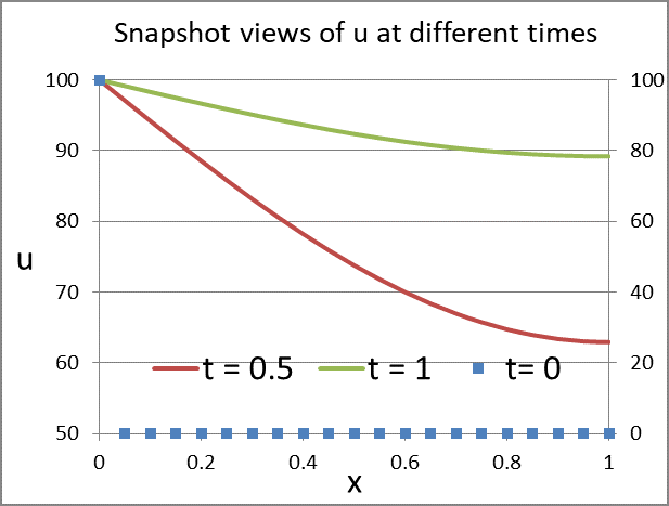
Next, we evaluate the array formula =PDSOLVE(B8, B2:B6, C8, D8, {0,1}, {0,1,2}) in allocated array G8:J30 and obtain the default snapshot-view formatted solution shown in Table 2. Figure 1 plots snapshot views of the temperature profiles at three time points.

The first argument B8 is a reference to the system RHS formula. the 2nd argument is a reference to the system variables. Alternatively, we could pass the equivalent defined names by combining them with Excel union operator as follows (t, x, u, ux, uxx) in argument 2. The 3rd and 4rth arguments are references to the left and right boundary conditions formulas.
We used Excel array constant syntax, {}, to pass the spatial domain [0, 1] in argument 5, and the time domain [0,1] in argument 6. Note that we have requested to report just 2 divisions in the output for the time interval [0,1] by using one of allowed formats for argument 6.

Table 2
	G	H	I	J
8	t	0	0.5	1
9	x	u	u	u
10	0	100	100	100
11	0.05	0	97.09061	99.15264
12	0.1	0	94.19917	98.31051
13	0.15	0	91.34352	97.47881
14	0.2	0	88.54128	96.66268
15	0.25	0	85.80973	95.86714
16	0.3	0	83.16573	95.09712
17	0.35	0	80.62557	94.35736
18	0.4	0	78.20491	93.65242
19	0.45	0	75.91868	92.98665
20	0.5	0	73.78095	92.36414
21	0.55	0	71.8049	91.78874
22	0.6	0	70.00271	91.26397
23	0.65	0	68.38546	90.79306
24	0.7	0	66.96312	90.37892
25	0.75	0	65.74445	90.02409
26	0.8	0	64.73694	89.73074
27	0.85	0	63.94682	89.50069
28	0.9	0	63.37894	89.33534
29	0.95	0	63.03681	89.23573
30	1	0	62.92253	89.20245

Optional Inputs

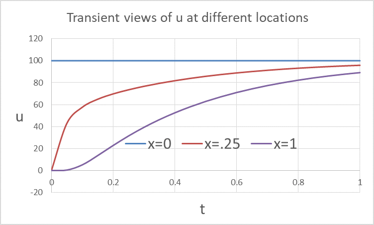
We can change the solution layout to display a transient format using the key FORMAT by evaluating the formula =PDSOLVE(B8, B2:B6, C8, D8, {0,1}, {0,1}, , {"FORMAT", "TCOL1"}) in array k4:O26. In this format, the locations of the spatial and time points are swapped as shown in Table 3. This permits easy plotting of transient views as shown in Figure 2. Note that we skipped over argument 7, and specified the optional key/value pair in argument 8 using a convenient array constant.

Table 3
	k	L	M	N	O
4	x	0	0.25	0.75	1
5	t	u	u	u	u
6	0	100	0	0	0
7	0.05	100	42.91949834	1.7783	0.313101
8	0.1	100	57.6237003	9.872125	5.069309
9	0.15	100	64.9427299	19.33831	13.57766
10	0.2	100	69.79061325	28.37773	22.76939
11	0.25	100	73.55257239	36.5845	31.45587
12	0.3	100	76.70668442	43.90968	39.32101
13	0.35	100	79.43829067	50.40811	46.33273
14	0.4	100	81.83335844	56.16036	52.55249
15	0.45	100	83.94479409	61.24727	58.05647
16	0.5	100	85.80973399	65.74445	62.92253
17	0.55	100	87.45722654	69.72003	67.22546
18	0.6	100	88.91220564	73.23462	71.03141
19	0.65	100	90.19820122	76.34145	74.39453
20	0.7	100	91.3353407	79.08748	77.36648
21	0.75	100	92.3413588	81.51442	79.99204
22	0.8	100	93.23124058	83.6594	82.31287
23	0.85	100	94.01741268	85.55562	84.36516
24	0.9	100	94.71177628	87.23199	86.18001
25	0.95	100	95.32502319	88.71406	87.78445
26	1	100	95.86714337	90.02409	89.20245

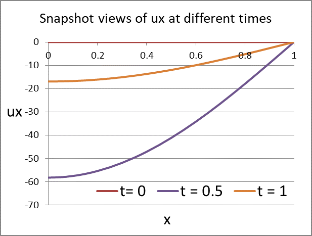
We can also request to output the derivative variables in the result using the key NDRVOUT. For example, to include ux in the output, we can evaluate the formula =PDSOLVE(B8, B2:B6, C8, D8, {0,1}, {0,1,2}, , {"NDRVOUT", 1}) in array A10:G32. The results are shown in Table 4 and Figure 3.

You can supply multiple control keys separated by commas using the constant array format as shown, or you can define them in a 2-column array and pass its address or name.

Table 4
	A	B	C	D	E	F	G
10	t	0	0	0.5	0.5	1	1
11	x	u	ux	u	ux	u	ux
12	0	100	0	100	-58.2477	100	-16.9647
13	0.05	0	0	97.09061	-58.068	99.15264	-16.9123
14	0.1	0	0	94.19917	-57.5301	98.31051	-16.7555
15	0.15	0	0	91.34352	-56.6371	97.47881	-16.4953
16	0.2	0	0	88.54128	-55.3948	96.66268	-16.1333
17	0.25	0	0	85.80973	-53.8108	95.86714	-15.6716
18	0.3	0	0	83.16573	-51.895	95.09712	-15.1134
19	0.35	0	0	80.62557	-49.6592	94.35736	-14.4618
20	0.4	0	0	78.20491	-47.1173	93.65242	-13.7212
21	0.45	0	0	75.91868	-44.2851	92.98665	-12.896
22	0.5	0	0	73.78095	-41.18	92.36414	-11.9914
23	0.55	0	0	71.8049	-37.8213	91.78874	-11.0131
24	0.6	0	0	70.00271	-34.2296	91.26397	-9.96694
25	0.65	0	0	68.38546	-30.4271	90.79306	-8.85955
26	0.7	0	0	66.96312	-26.4373	90.37892	-7.69767
27	0.75	0	0	65.74445	-22.2846	90.02409	-6.48848
28	0.8	0	0	64.73694	-17.9947	89.73074	-5.23936
29	0.85	0	0	63.94682	-13.594	89.50069	-3.95803
30	0.9	0	0	63.37894	-9.10946	89.33534	-2.6523
31	0.95	0	0	63.03681	-4.56882	89.23573	-1.33025
32	1	0	0	62.92253	-1.8E-12	89.20245	-1.8E-12

Example 2: Solving a nonlinear coupled PDE system

The following coupled nonlinear system has known analytical solution for the following configuration:

\frac{\partial u}{\partial t} = u_{x} v_{x} + (v - 1) u_{x x} + (16 x . t - 2 t - 16 (v - 1)) (u - 1) + 10 x . e^{- 4 x}

\frac{\partial v}{\partial t} = v_{x x} + u_{x} + 4 u - 4 + x^{2} - 2 t - 10 t . e^{- 4 x}

Time period	`t ∈` [0,2]
Spatial range	`0 ≤ x ≤ 1`
Initial values	$u (x, 0) = 1$ $v (x, 0) = 1$
Left boundary condition	$u (0, t) = 1$ $v (0, t) = 1$
Right boundary condition	$u_{x} (1, t) = 3 (1 - u (1, t))$ $v_{x} (1, t) = 0.2 (u (1, t) - 1) e^{4}$

The exact solution¹ is given by:

u (x, t) = 1 + 10 x . t . e^{- 4 x}

v (x, t) = 1 + x^{2} t

¹Madsen N.K., Sincovec R.F. Software for partial differential equations, in Numerical Methos for Differential Systems, L. Lapidus, W.E. Schiesser eds., Acedemic Press, New York (1976))

We solve this system next with PDSOLVE

Solution

Working with the named variables t, x, u, v, ux, vx, uxx, vxx, we define the input arguments to PDSOLVE as shown in Table 1, including the system equations, left and right boundary conditions formulas, and the initial values for u and v.

Table 1
	A	B	C	D
1	Variables
2	t		ux
3	x		vx
4	u	1	uxx
5	v	1	vxx
6	Equations		Left Bc	Right Bc
7	u,t	=vxux+(v-1)uxx+(16xt-2t-16(v-1))(u-1)+10xEXP(-4x)	=u-1	=ux-3*(1-u)
8	v,t	=vxx+ux+4u-4+x^2-2t-10tEXP(-4*x)	=v-1	=vx-0.2(u-1)EXP(4)

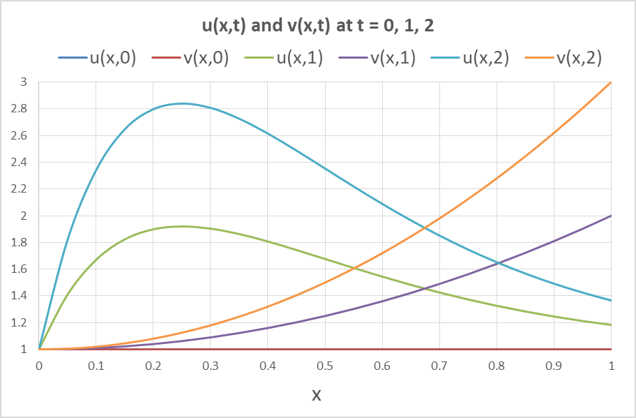
To obtain the solution, we evaluate the formula =PDSOLVE(B7:B8, (B2:B5,D2:D5), C7:C8, D7:D8, {0,1}, {0,1}) in allocated array A10:G32 and obtain the solution shown in Table 2. The numerical results are virtually identical to the analytical solution with shown precision. Snapshots of u and v profiles at different times are plotted in Figure 1.

Excel Tip. We used Excel union operator (Ref1, Ref2, ..), to combine all the system variables (B2:B5,D2:D5) into one reference in argument 2. The union operator preserves the order of the variables which is required. This is equivalent to grouping the named variables in the required order (t, x, u, v, ux, vx, uxx, vxx) in argument 2.

Table 2
	A	B	C	D	E	F	G
10	t	0	0	1	1	2	2
11	x	u	v	u	v	u	v
12	0	1	1	1	1	1	1
13	0.05	1	1	1.409366	1.0025	1.818731	1.005
14	0.1	1	1	1.67032	1.01	2.340639	1.02
15	0.15	1	1	1.823218	1.0225	2.646435	1.045
16	0.2	1	1	1.898658	1.04	2.797316	1.08
17	0.25	1	1	1.919699	1.0625	2.839397	1.125
18	0.3	1	1	1.903583	1.09	2.807166	1.18
19	0.35	1	1	1.863089	1.1225	2.726179	1.245
20	0.4	1	1	1.807586	1.16	2.615172	1.32
21	0.45	1	1	1.743845	1.2025	2.48769	1.405
22	0.5	1	1	1.676676	1.25	2.353353	1.5
23	0.55	1	1	1.609417	1.3025	2.218835	1.605
24	0.6	1	1	1.544308	1.36	2.088616	1.72
25	0.65	1	1	1.482778	1.4225	1.965557	1.845
26	0.7	1	1	1.42567	1.49	1.851341	1.98
27	0.75	1	1	1.373403	1.5625	1.746806	2.125
28	0.8	1	1	1.326098	1.64	1.652195	2.28
29	0.85	1	1	1.283673	1.7225	1.567346	2.445
30	0.9	1	1	1.245914	1.81	1.491827	2.62
31	0.95	1	1	1.212522	1.9025	1.425045	2.805
32	1	1	1	1.183156	2	1.366313	3

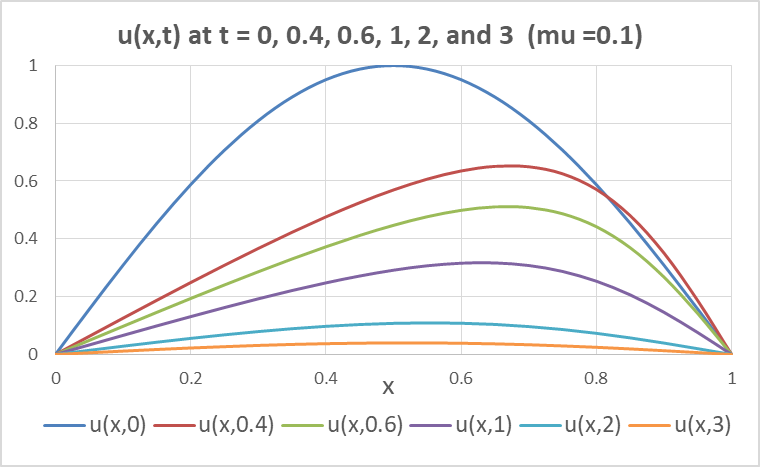
Example 3: Solving Burgeres equation

Burgers equation arises in various topics including fluid mechanics in particular.

\frac{\partial u}{\partial t} = - u \frac{\partial u}{\partial x} + v \frac{\partial^{2} u}{\partial x^{2}}

We solve this system for the following configuration and compare our numerical results with published exact Fourier solution

Time period	`t ∈` [0,3]
Spatial range	`0 ≤ x ≤ 1`
Parameter	`μ = 0.1 and .01`
Initial value	$u (x, 0) = \sin (π x)$
Left boundary condition	$u (0, t) = 0$
Right boundary condition	$u (1, t) = 0$

Solution

Working with named variables t, x, u, ux, uxx, we define the input arguments to PDSOLVE as shown in Table 1, including the system equation, left and right boundary conditions formulas, and the initial value for u.

Table 1
	A	B	C	D
1	Variables		Parameters
2	t		mu	0.1
3	x
4	u	=SIN(PI()*x)
5	ux
6	uxx
7	Equations		Left Bc	Right Bc
8	du/dt	=muuxx-uux	=u	=u

Next, we evaluate the array formula =PDSOLVE(B8, B2:B6, C8, D8, {0,1}, {0,0.4,0.6,1,2,3}) in allocated array A10:G32 and obtain the solution shown in Table 2. Note that we have requested to report custom output time points in the interval [0,3] using one of the allowed formats for argument 6. Figure 1 plots snapshot views of the u at various time points.

Table 2
	A	B	C	D	E	F	G
10	t	0	0.4	0.6	1	2	3
11	x	u	u	u	u	u	u
12	0	0	-1.09849E-19	-1.76817E-19	-3.38039E-19	-6.94334E-19	-7.66987E-19
13	0.05	0.156434	0.062967368	0.048911187	0.033239453	0.014479494	0.00591558
14	0.1	0.309017	0.125652393	0.09764422	0.066311545	0.028753611	0.011711215
15	0.15	0.45399	0.187759988	0.146009437	0.09903539	0.042612425	0.017267755
16	0.2	0.587785	0.248967988	0.1937925	0.131201781	0.055837184	0.022467765
17	0.25	0.707107	0.308909449	0.240737705	0.162555919	0.068196653	0.027196686
18	0.3	0.809017	0.367148979	0.286525231	0.192776238	0.079444482	0.031344339
19	0.35	0.891007	0.423149575	0.330738977	0.221448139	0.089318163	0.034806865
20	0.4	0.951057	0.476224634	0.372820357	0.248031646	0.097540284	0.037489146
21	0.45	0.987688	0.52546721	0.412001795	0.271822782	0.103822939	0.039307725
22	0.5	1	0.569646198	0.447213154	0.291910985	0.107876231	0.040194162
23	0.55	0.987688	0.607055139	0.476953781	0.307137937	0.109421761	0.04009872
24	0.6	0.951057	0.635303383	0.499131496	0.316071605	0.108211614	0.038994127
25	0.65	0.891007	0.651049314	0.510885043	0.317017903	0.10405284	0.036879198
26	0.7	0.809017	0.649727143	0.508454577	0.308107184	0.096835993	0.033781846
27	0.75	0.707107	0.625420424	0.487238594	0.28750007	0.086565254	0.029761188
28	0.8	0.587785	0.571236655	0.442286995	0.253749775	0.073385482	0.024908229
29	0.85	0.45399	0.48074178	0.369527647	0.206311494	0.057600781	0.019344871
30	0.9	0.309017	0.350911318	0.267818401	0.146094008	0.039678638	0.013220984
31	0.95	0.156434	0.186022413	0.141222145	0.075829949	0.020235104	0.006709534
32	1	1.23E-16	1.22515E-16	1.22515E-16	1.22515E-16	1.22515E-16	1.22515E-16

Effect of viscosity μ

We change the value of mu in D2 from 0.1 to 0.01. Figure 2 shows the updated profiles for u.

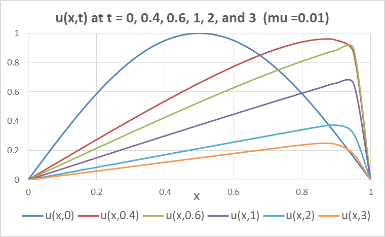
Comparison with published analytical solution

A Fourier-based solution¹ values for Burgers equation for two values of μ are listed in Table 3 along with computed values by PDSOLVE. The results are virtually identical.

¹S. Kutluay, A.R. Bahadir, A. Ozdes, Numerical solution of one-dimensional Burgers equation, explicit and exact-explicit finite difference method. Journal of Computational and Applied Mathematics 103 (i 999) 251-261

Table 3
x	`t`	`u` (μ=0.1) Fourier PDSOLVE	`u` (μ=0.01) Fourier PDSOLVE
0.25	0.6	0.24074 0.240737705	0.26896 0.268975372
	1	0.16256 0.162555919	0.18819 0.188198472
	3	0.02720 0.027196686	0.07511 0.075115705
0.75	0.6	0.48721 0.487238594	0.76724 0.767275326
	1	0.28747 0.28750007	0.55605 0.556072119
	3	0.02977 0.029761188	0.22481 0.224816515

Algorithms

PDSOLVE implements the method of lines. Spatial discretization is carried out on a uniform mesh using a standard collocation method. The resulting implicit ODE system is integrated by any of the algorithms RADAU5, BDF, or ADAMS with adaptive step control.

BDF: An implicit backward differentiation formula method (DLSODE) suitable for nonlinear stiff and non-stiff systems. (Default algorithm.)
RADAU5: An implicit Runge-Kutta method of order 5 with adaptive step size and error control. suitable for nonlinear stiff problems.
ADAMS: An implicit Adams method (DLSODI) suitable for non-stiff systems.

References

Schiesser W.E (1991). The Numerical Method of Lines, San Diego, CA: Academic Press, 1991.
Ascher U M, Mattheij R M M and Russell R D. Numerical Solution of Boundary Value Problems for Ordinary Differential Equations, Prentice Hall, (1988).
Ernst Hairer and Gerhard Wanner, Solving Ordinary Differential Equations II: Stiff and Differential-Algebraic Problems (Springer Series in Computational Mathematics), 1996.
Alan C. Hindmarsh, ODEPACK, A Systematized Collection of ODE Solvers, in Scientific Computing, R. S. Stepleman et al. (Eds.), North-Holland, Amsterdam, 1983, pp. 55-64.

ExcelWorks LLC

Solving Partial Differential Equations in Excel

Syntax

=PDSOLVE(eqns, vars, lbc, rbc, xdom, tdom, [options])

Initial Conditions

Boundary Conditions

Required Inputs

Optional Inputs

Snapshot View Format

Transient View Format

Solution

Optional Inputs

Solution

Solution

Effect of viscosity μ

Comparison with published analytical solution

`=PDSOLVE(eqns, vars, lbc, rbc, xdom, tdom, [options])`