
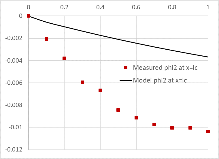
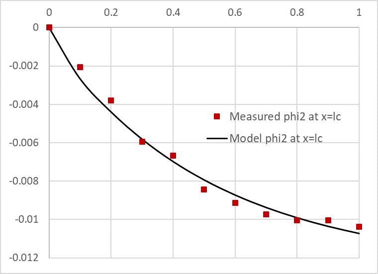
This example will show you how to solve a complex system of PDEs, then optimize the system parameters to obtain excellent fit with experimental data. We will first obtain a solution using default values for the parameters with PDASOLVE (Figure a), then optimize the model using Excel Solver or NLSOLVE (Figure b).
For a detailed description of this problem, please see Example 1 of PDASOLVE
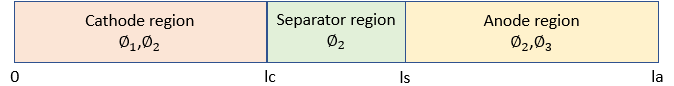
| x = 0 | x = lc | x = ls | x = la |
|---|---|---|---|
Working with named system variables, parameters, and property functions we define the complete Excel model including equations, regions, and boundary conditions formulas as shown in Table 1.
| A | B | C | D | E | F | G | H | |
| 1 | System Variables with initial values | System Parameters | ||||||
|---|---|---|---|---|---|---|---|---|
| 2 | t | lc | 2.00E-04 | |||||
| 3 | x | ls | 2.254E-04 | |||||
| 4 | phi_1 | 0 | la | 4.254E-04 | ||||
| 5 | phi_2 | 0 | beta | 1 | ||||
| 6 | phi_3 | 0 | gamma | 0.5 | ||||
| 7 | phi1x | mc | 1E+06 | |||||
| 8 | phi2x | |||||||
| 9 | phi3x | Mass Matrix | ||||||
| 10 | phi1xx | 1E+06 | =-mc | 0 | ||||
| 11 | phi2xx | =-mc | 1E+06 | =-mc | ||||
| 12 | phi3xx | 0 | =-mc | 1E+06 | ||||
| 13 | ||||||||
| 14 | Property Functions | x Domain | 0 | =la | ||||
| 15 | sigma | =IF(x<=lc,1,IF(x<ls,0,1)) | t Interval | 0 | 1 | Boundary conditions matrix | ||
| 16 | kappa | =beta*IF(x<=lc,1,IF(x<ls,2,1)) | 0 | R | =sigma*phi1x-1 | |||
| 17 | a | =gamma*IF(x<=lc,1E6,IF(x<ls,0,1E6)) | 0 | N | =phi2x | |||
| 18 | f | =IF(x<=lc,3*EXP(-2*t),0) | =lc | N | =phi1x | |||
| 19 | =lc | C | =kappa*phi2x | |||||
| 20 | System RHS Equations | Regions | =ls | C | =kappa*phi2x | |||
| 21 | eq1 | =sigma*phi1xx-a*(phi_1-phi_2-f) | 0 | =lc | =ls | N | =phi3x | |
| 22 | eq2 | =kappa*phi2xx+a*(phi_1-phi_2-f) | 0 | =la | =la | N | =phi2x | |
| 23 | eq3 | =sigma*phi3xx-a*(phi_3-phi_2-f) | =ls | =la | =la | D | =phi_3 | |
To aid readability, we assign assign names for selected Excel ranges in Table 1 which represent input arguments to PDASOLVE as shown in Table 2.
| Excel Range | Assigned Name |
|---|---|
| B21:B23 | Eqns |
| B2:B12 | Vars |
| F16:H23 | BCs |
| D14:E14 | xDom |
| D15:E15 | tDom |
| C10:E12 | M |
| C21:D23 | Rgns |
Next, we evaluate the array formula
=PDASOLVE(Eqns, Vars, BCs, xDom, tDom, M, Rgns, , {"FORMAT","TCOL1"})
in array G15:S27 and obtain the solution as shown in Table 3.
| G | H | I | J | K | L | M | N | O | P | Q | R | S | |
| 15 | x | 0 | 0 | 0 | 0.0002 | 0.0002 | 0.0002 | 0 | 0.0002254 | 0.0002254 | 0.0004254 | 0.0004254 | 0.00043 |
| 16 | t | phi_1 | phi_2 | phi_3 | phi_1 | phi_2 | phi_3 | phi_1 | phi_2 | phi_3 | phi_1 | phi_2 | phi_3 |
| 17 | 0 | 0 | 0 | 0 | 0 | 0 | 0 | 0 | 0 | 0 | 0 | 0 | 0 |
| 18 | 0.1 | 0.0490406 | -0.0031269 | 0 | 0.0491381 | -0.0026646 | 0 | 0 | -0.0026093 | -0.0003937 | 0 | -0.002235 | 0 |
| 19 | 0.2 | 0.0888748 | -0.004782 | 0 | 0.0889728 | -0.0043945 | 0 | 0 | -0.0043481 | -0.0003311 | 0 | -0.004033 | 0 |
| 20 | 0.3 | 0.1204078 | -0.0061393 | 0 | 0.1205061 | -0.0058129 | 0 | 0 | -0.0057737 | -0.0002801 | 0 | -0.005507 | 0 |
| 21 | 0.4 | 0.1451792 | -0.0072539 | 0 | 0.1452778 | -0.0069774 | 0 | 0 | -0.0069442 | -0.0002385 | 0 | -0.006716 | 0 |
| 22 | 0.5 | 0.1644121 | -0.0081697 | 0 | 0.164511 | -0.0079339 | 0 | 0 | -0.0079055 | -0.0002046 | 0 | -0.00771 | 0 |
| 23 | 0.6 | 0.1791579 | -0.0089244 | 0 | 0.179257 | -0.0087217 | 0 | 0 | -0.0086973 | -0.0001769 | 0 | -0.008528 | 0 |
| 24 | 0.7 | 0.1902228 | -0.0095468 | 0 | 0.190322 | -0.0093711 | 0 | 0 | -0.0093499 | -0.0001544 | 0 | -0.009201 | 0 |
| 25 | 0.8 | 0.1983065 | -0.0100621 | 0 | 0.1984059 | -0.0099083 | 0 | 0 | -0.0098896 | -0.0001361 | 0 | -0.009758 | 0 |
| 26 | 0.9 | 0.2039649 | -0.01049 | 0 | 0.2040644 | -0.010354 | 0 | 0 | -0.0103374 | -0.0001213 | 0 | -0.01022 | 0 |
| 27 | 1 | 0.2076535 | -0.0108468 | 0 | 0.2077531 | -0.0107253 | 0 | 0 | -0.0107105 | -0.0001093 | 0 | -0.010605 | 0 |
In Figure 1, we plot phi2(x,t) at the interface x = lc together with imperical values for Φ(lc,t). Clearly the default model does not agree well with experimental data. Next will show you how to optimize the model parameters so it agrees with experimental data accurately.
The observed experimental values for Φ(lc,t) are give in Table 6.
| M | N | |
| 1 | time | Emperical phi2 |
|---|---|---|
| 2 | 0 | 0 |
| 3 | 0.1 | -0.002052705 |
| 4 | 0.2 | -0.00380538 |
| 5 | 0.3 | -0.005944579 |
| 6 | 0.4 | -0.006668727 |
| 7 | 0.5 | -0.008436437 |
| 8 | 0.6 | -0.009136398 |
| 9 | 0.7 | -0.009734491 |
| 10 | 0.8 | -0.010031262 |
| 11 | 0.9 | -0.010050529 |
| 12 | 1 | -0.010387955 |
Our task is to compute optimal values for the design parameters γ, and mc which minimize the sum of square residuals between our model predictions and the observed data in Table 6. We have two options to solve this dynamical minimization problem: Excel native Solver, and NLSOLVE. We demonstrate both procedures below.
We define an objective formula to be minimized. The objective formula calculates the summation of the square residuals between the observed values and their corresponding computed values from the solution result in Table 3. The definition of the objective formula is shown in S2 of Table 7 with initial value of 0.00033.
| P | S | |
| 1 | =(L18-N2)^2 | Objective |
|---|---|---|
| 2 | =(L19-N3)^2 | =SUM(P1:P10) |
| 3 | =(L20-N4)^2 | |
| 4 | =(L21-N5)^2 | |
| 5 | =(L22-N6)^2 | |
| 6 | =(L23-N7)^2 | |
| 7 | =(L24-N8)^2 | |
| 8 | =(L25-N9)^2 | |
| 9 | =(L26-N10)^2 | |
| 10 | =(L27-N11)^2 | |
| 10 | =(L28-N12)^2 |
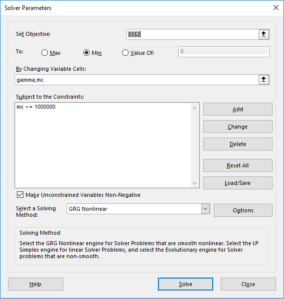
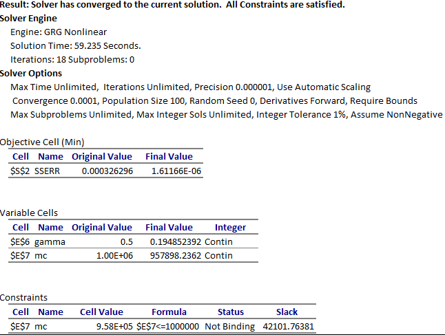
The remaining task is to configure and run Excel Solver command. We configure the solver exactly as shown in Figure 2. We select to minimize the objective formula S2, by varying gamma and mc, subject to the upper bound constraint mc <= 10e6 which is added for numerical stability since larger values for the off-diagonal mass matrix element mc leads to a divergent system.
We run the solver which reports a feasible solution in less than a minute of computing time as shown in the Answer Report generated by the Excel Solver in Figure 3. Upon accepting the solution, Excel automatically updates the spreadsheet to reflect the optimal computed values. The optimized solution for phi2 is shown in Figure 4 exhibiting excellent agreement with observed values.
NLSOLVEUnlike Excel Solver which requires an objective formula, NLSOLVE requires the list of individual residual constraint formulas which we define as shown in Table 8.
| R | |
| 1 | =DYNVAL(L18)-N2 |
| 2 | =DYNVAL(L19)-N3 |
| 3 | =DYNVAL(L20)-N4 |
| 4 | =DYNVAL(L21)-N5 |
| 5 | =DYNVAL(L22)-N6 |
| 6 | =DYNVAL(L23)-N7 |
| 7 | =DYNVAL(L24)-N8 |
| 8 | =DYNVAL(L25)-N9 |
| 9 | =DYNVAL(L26)-N10 |
| 10 | =DYNVAL(L27)-N11 |
| 10 | =DYNVAL(L27)-N12 |
Note that we use DYNVAL to select values from the solution array because we want to use their dynamic values during the optimization.
Please note. DYNVAL is a new function available in ExceLab 7.0 and later versions only. It replaces deprecated Criterion Functions used in earlier versions.
Next, we evaluate the formula =NLSOLVE(R1:R10, (gamma, mc)) in array S4:T8 and obtain virtually the same solution found by Excel Solver
as shown in Table 9. However, NLSOLVE, converges in fewer iterations in less than one third of the time.
Since NLSOLVE is a pure spreadsheet function, it does not modify its arguments.
Therefore, to update the spreadsheet result, the computed values for gamma and mc are copied manually to
their respective variable cells D6 and D7 of Table 3 of Example 1.
| S | T | |
| 4 | gamma | 0.195638747 |
| 5 | mc | 958050.8287 |
| 6 | SSERROR | 1.61147E-06 |
| 7 | ITRN | 10 |
| 8 | TIME (s) | 18.729 |
Ghaddar, C.K. "Rapid Modeling and Parameter Estimation of Partial Differential Algebraic Equations by a Functional Spreadsheet Paradigm". Math. Comput. Appl. 2018, 23, 39.
Available at: http://www.mdpi.com/2297-8747/23/3/39