ExcelWorks LLC

Computing Train Travel Time and Thrust

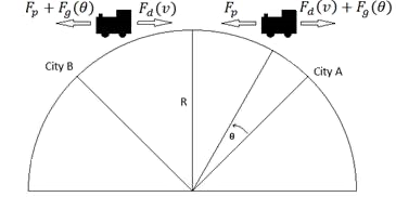
Consider a frictionless train that uses a constant propulsion force to accelerate but relies solely on the gravitational pull of the Earth and aerodynamic drag for deceleration.  Using the simplifying assumption shown in Table 1, we compute the required propulsion force and the travel time for the train between two cities 1000km  apart through a straight tunnel.

Problem Formulation

Figure 1 shows the forces  acting on the train during its trip from City A to City B along the earth circular path.

The motion for the train is governed by the 2^nd order equation:

mx¨=Fp-Fdx˙+Fgθx

where θ(x), can be approximated by the following function based on the fact that d/r << 1

θx=tan-1Rd2-x,x<d2π2,x=d2tan-1Rd2-x+π,x>d2

The train starts from rest so the initial values are:

x0=0 x˙0=0

Upon arrival to city B, the train would have travelled distance d and come to a stop so the final conditions can be stated as:

x<msub><mi>t</mi><mi>f</mi></msub>=d x˙tf=0

The unknown variables for this problem are F_p and t_f which we need to solve for.

Solution

We treat the final conditions as constraints on the equation of motion then solve for the unknown variables F_p and t_f to satisfy them. We accomplish our task following a simple three-step dynamical optimization procedure.

Step 1: siumlate the initial value problem using guess values for the unknowns

The first step is to convert the 2nd order equation into two first order equations as follows:

$$\frac{dx}{dt}=v$$ $$\frac{dv}{dt}=\frac{1}{m}\left(F_p-F_d\left(\dot{x}\right)+F_g\left(\theta \left(x\right)\right)\right)$$

Next, we define the model formulas using the named variables as shown in Table 2. The green, B2:B4, and yellow, B11:B12, ranges represent the system variables (t,x,v), and the differential equations which are input arguments to the initial value problem solver function, IVSOLVE. The blue, D10:D11 range represents the design parameters F_p and t_f which have been assigned initial guess values of 1000 and 2000 respectively. The other named variables and formulas in Table 2 are auxiliary variables to simplify the definition the model equations.

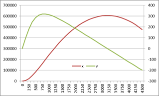
We simulate the system with the guess value for a sufficient long time of 4500 seconds by executing the array formula =IVSOLVE(B11:B12, (t,x,v), {0,4500}) in array J3:L40 shown in Table 3 and plotted in Figure 2.

Step 2: define constraints on the initial solution.

In Table 4, we define two constraints corresponding to the final conditions x<msub><mi>t</mi><mi>f</mi></msub>=d and x˙tf=0 based on the solution obtained in Step 1. Constraint C10 computes the difference between the interpolated value for x(t_f) and the distance d, while constraint C11 computes the interpolated value for v(t_f).

Here we are simply computing values x(t_f) and v(t_f) using INTERPXY based on the result in Table 3. Note that we use DYNVAL to select the displacement and velocity columns from the solution array because we want to use their dynamic values during the optimization. The time column values are static, therefore, we can select its values directly.

Please note. DYNVAL is a new function available in ExceLab 7.0 and later versions only. It replaces deprecated Criterion Functions used in earlier versions.

Step 3: solve for the unknowns

Using the solver NLSOLVE, we solve for the unknowns t_f and F_p by evaluating the array formula =NLSOLVE(C10:C11, (tf, Fp)) in array A10:B14. The computed results are shown in Table 5. NLSOLVE finds the best values for the variables which drive the constraint formulas values simultaneously to zero.