The above classical textbook equation describes a 2nd order dynamical system. In this formulation, x(t) represents the displacement, ω represents the natural frequency, and ζ represents the damping ratio. To simulate this system with IVSOLVE, we transform it to two first order equations:
Using the named variables and initial values, we define the input to IVSOLVE as shown in Table 1.
| A | B | C | D | |
| 1 | Variables with initial values | Parameters | ||
|---|---|---|---|---|
| 2 | t | omega | 1 | |
| 3 | x | 1 | zeta | 0.25 |
| 4 | v | 0 | ||
| 5 | Equations | |||
| 6 | dx/dt | =v | ||
| 7 | dv/dt | =-2*zeta*omega*v-omega^2*x | ||
Next, we evaluate the array formula =IVSOLVE(B6:B7, (t,x,v), {0,12}) in array I1:K41
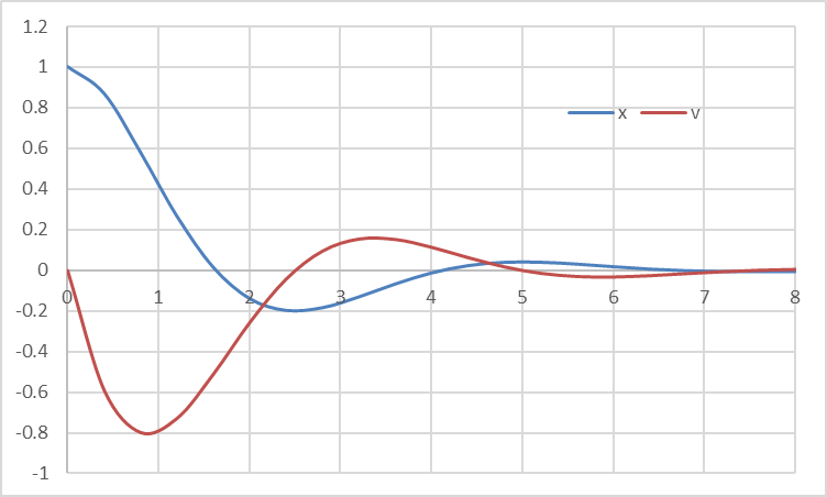
and obtain the solution shown Table 2 and plotted in Figure 1.
Note. ExceLab 365 users pass system variables by range reference B2:B4 or as "(t,x,v)" . Google Sheets users pass by range reference or as {t,x,v}
| I | J | K | |
| 1 | t | x | v |
| 2 | 0 | 1 | 0 |
| 3 | 0.4 | 0.926057 | -0.35295 |
| 4 | 0.8 | 0.733004 | -0.59143 |
| 5 | 1.2 | 0.470053 | -0.70204 |
| 6 | 1.6 | 0.187507 | -0.69215 |
| 7 | 2 | -0.07064 | -0.585 |
| 8 | 2.4 | -0.2719 | -0.41357 |
| 9 | 2.8 | -0.39777 | -0.21403 |
| 10 | 3.2 | -0.4439 | -0.02004 |
| 11 | 3.6 | -0.41815 | 0.14165 |
| 12 | 4 | -0.33723 | 0.253773 |
| 13 | 4.4 | -0.22273 | 0.309249 |
| 14 | 4.8 | -0.09711 | 0.31042 |
| 15 | 5.2 | 0.019632 | 0.26696 |
| 16 | 5.6 | 0.112406 | 0.193178 |
| 17 | 6 | 0.172275 | 0.10513 |
| 18 | 6.4 | 0.19664 | 0.018001 |
| 19 | 6.8 | 0.188456 | -0.05592 |
| 20 | 7.2 | 0.154784 | -0.10843 |
| 21 | 7.6 | 0.105069 | -0.13591 |
| 22 | 8 | 0.049333 | -0.13896 |
| 23 | 8.4 | -0.00336 | -0.12157 |
| 24 | 8.8 | -0.04602 | -0.08994 |
| 25 | 9.2 | -0.07437 | -0.05117 |
| 26 | 9.6 | -0.08693 | -0.01211 |
| 27 | 10 | -0.08478 | 0.021603 |
| 28 | 10.4 | -0.07088 | 0.046117 |
| 29 | 10.8 | -0.04936 | 0.059586 |
| 30 | 11.2 | -0.02468 | 0.062088 |
| 31 | 11.6 | -0.00094 | 0.055252 |
| 32 | 12 | 0.018627 | 0.041749 |
The solution shows that the system is underdamped with an absolute overshoot over 0.4 at approximately a peak time of 3.3. In this exercise, we will customize the system response by optimizing ζ and ω to achieve an absolute overshoot of exactly 0.2 at t = 2.0.
We define two constraints on the solution obtained in Table 2 to demand that x(2) = -0.2 and v(2) = 0, then use NLSOLVE to solve for ω and ζ that staisfy these constraints. The two constraint formulas are shown in Table 3.
| C | |
| 1 | =DYNVAL(J7)-(-0.2) |
| 2 | =DYNVAL(K7) |
J7 and K7 refer to x(2)
and v(2) values respectively from the solution array shown in Table 2. Note that we use DYNVAL to select the values from the solution array.
DYNVAL is a dummy function that simply returns the value of its argument but in this context, it ensures that its argument is dynamically evaluated during the optimization.
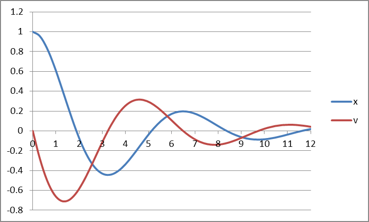
We evaluate the array formula =NLSOLVE(C1:C2, (omega, zeta)) in array D1:E5 and obtain the solution
shown in Table 4 and plotted in Figure 2. The new solution has an absolute overshoot of 0.2 at t=2 as desired.
Note. ExceLab 365 users pass omega and zeta variables by range reference D2:D3. Google Sheets users pass by range reference or as {omega,zeta}
| D | E | |
| 1 | omega | 1.76493157 |
| 2 | zeta | 0.455950294 |
| 3 | SSERROR | 7.61331E-12 |
| 4 | ITRN | 11 |
| 5 | TIME(s) | 0.283 |
What if we wanted our peak time to be at 2.5 instead of 2. Our solution array in Table 1 does not list the output point t=2.5. We have two options:
We can format the output to display the solution at t=2.5 (See Output Format section in IVSOLVE help page).
We modify the constraint formulas in Table 3 by employing INTERPXY to interpolate x and v at t = 2.5 as shown in Table 5.
| C | |
| 1 | =INTERPXY(I2:I32,DYNVAL(J2:J32),2.5)-(-0.2) |
| 2 | =INTERPXY(I2:I32,DYNVAL(K2:K32),2.5) |
Note that we use DYNVAL to select the displacement and velocity columns from the solution array because we want to use their dynamic values during the optimization.
The time column values are static, therefore, we can select its values directly.
Please note. DYNVAL is a new function available in ExceLab 7.0 and later versions only. It replaces deprecated Criterion Functions used in earlier versions.
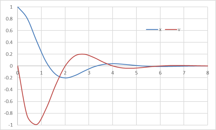
Using the same formula but with updated constraint formulas, NLSOLVE computes the new solution shown in table 6 Below and plotted in Figure 3. Note that the peak time has shifted to 2.5.
| D | E | |
| 1 | omega | 1.411995975 |
| 2 | zeta | 0.455958508 |
| 3 | SSERROR | 1.55938E-25 |
| 4 | ITRN | 8 |
| 5 | TIME(s) | 0.152 |