The first example describes a bang-bang (two-stage) control problem . The mathematical problem is stated as follows:
Minimize |
|
|---|---|
|
|
(1) |
subject to |
|
|
|
(2) |
|
|
(3) |
|
|
(4) |
|
|
(5) |
Working with named variables shown in Table 1, we parametrized the two-stage control function, u(t), using a standard IFstatement,
as shown in B9. The unknown parameters switchT, stage1, and stage2 are assigned the initial guess values 0.1, 0, and 1.
We define the formulas for the ODE equations (2) and (3) in B11 and B12, and assign the initail values (4) to x and y in
in B3 and B4.
| A | B | |
| 1 | ODE variables | |
| 2 | t | 0 |
| 3 | x | 0.231 |
| 4 | y | 1.126 |
| 5 | Parametrized control formula | |
| 6 | switchT | 0.1 |
| 7 | stage1 | 0 |
| 8 | stage2 | 1 |
| 9 | u | =IF(t<=switchT,stage1,stage2) |
| 10 | ODE rhs formulas | |
| 11 | xdot | =y |
| 12 | ydot | =u−x+y |
We obtain a solution to the inner initial value problem by evaluating the array formula =IVSOLVE(B11:B12, B2:B4, {0,5}) in an allocated array D2:F103.
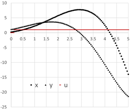
The result is shown partially in Table 2, and the initial trajectories of x(t), y(t), and u(t) are plotted in Figure 1.
| D | E | F | H | J | L | M | |
| 1 | IVP Solution | ||||||
|---|---|---|---|---|---|---|---|
| 2 | t | x | y | u | Integrand | Cost functional | |
| 3 | 0 | 0.231 | 1.126 | 0 | 1.321237 | Objective | 246.0854 |
| 4 | 0.05 | 0.288414 | 1.170438 | 0 | 1.453107 | ||
| 5 | 0.1 | 0.348032 | 1.21424 | 0 | 1.595504 | Constraint formulas | |
| 6 | 0.15 | 0.411089 | 1.308339 | 1 | 1.880744 | Max(u) | 1 |
| 7 | 0.2 | 0.478891 | 1.403911 | 1 | 2.200301 | Min(u) | 0 |
| 102 | 4.95 | −12.9106 | −21.0491 | 1 | 609.7477 | ||
| 103 | 5 | −13.9717 | −21.3881 | 1 | 652.6612 | ||
| Purpose | Cell | Formula |
|---|---|---|
| Initial value problem solution | D2:F103 | =IVSOLVE(B11:B12, B2:B4, {0,5}) |
| AutoFill formula for control values | H3 | =IF(D3<=switchT, stage1, stage2) |
| AutoFill formula for integrand values | J3 | =E3^2+F3^2 |
| Objective formula | M3 | =0.5*QUADXY(D3:D103, J3:J103) |
| Maximum value of control column | M6 | =MAXA(H3:H103) |
| Minimum value of control column | M7 | =MINA(H3:H103) |

To define the objective formula for the cost functional (1), we generate, based on the obtained initial solution in Table 2, two columns for the control function and the integrand expression using formulas H3 and J3 shown in Table 3. Next, we define the objective formula M3 in which we use QUADXY to integrate the integrand column versus the solution output times column. The initial value of the objective formula is 246.0854, as shown in Table 2.
To impose the bound constraint (5) on u(t), we defined two aid formulas in M6 and M7 which computed the maximum and minimum of the generated control column values. We make use of these aid formulas during the configuration of Excel Solver.
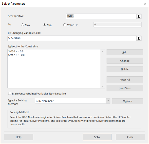
We configure Excel Solver as shown in Figure 2 to minimize the objective formula M3 by varying the control parameters B6:B8 (corresponding to switchT, stage1 and stage2) subject to the constraints
|
M6 ≤ 0.8 corresponds to max(u) ≤ 0.8, |
|
|
M7 ≥ −0.8 corresponds to min(u) ≥ −0.8, |
which are needed to impose (5). We uncheck the box which reads 'Make Unconstrained Variables Non-Negative' to allow the variables to take on negative values as well. In the options for the GRG Nonlinear solver, we switch the derivative scheme from the default Forward to Central, and then run the Solver.

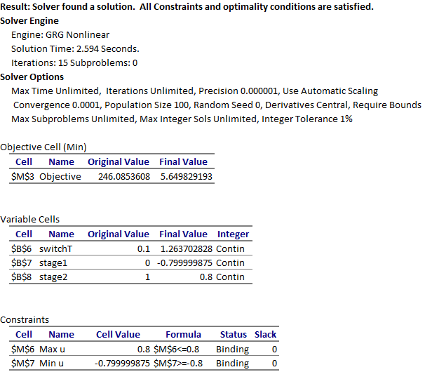
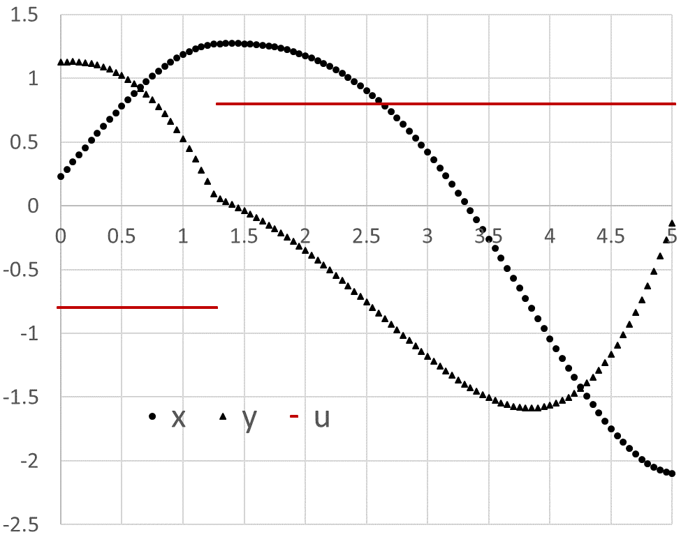
Excel Solver reports a feasible solution in less than 3 seconds and generates an Answer Report shown in Figure 3. The optimal switching time is found at approximately 1.26 which is within 1% of the 1.25 value reported by Elnagar and Kazemi [1] using a pseudo-spectral Chebyshev approximation of order 15. The optimal trajectories are plotted in Figure 4.


[1] Elnagar, G.; Kazemi, M.A. Pseudospectral Chebyshev Optimal Control of Constrained Nonlinear Dynamical Systems. Comput. Optim. Appl. 1998, 11, 195-217.
[2] Ghaddar, C. K. "Novel Spreadsheet Direct Method for Optimal Control Problems." Math. Comput. Appl., 23, 6, 2018.
Available at: http://www.mdpi.com/2297-8747/23/1/6
[3] Ghaddar, C.K. "Rapid Solution of Optimal Control Problems by a Functional Spreadsheet Paradigm: A Practical Method for the Non-Programmer". Math. Comput. Appl. 2018, 23, 54.
Available at: https://www.mdpi.com/2297-8747/23/4/54