
This problem considers the optimal control of a fed-batch reactor for the production of ethanol [1]. The goal is to maximize the yield of ethanol using the feed rate as the control. Unlike the previous examples, this problem has a free terminal time tF, which is also an unknown design variable. The mathematical statement of the problem is given below:
Find the flowrate u(t), and the terminal time tF which
|
maximize the cost index |
|
|---|---|
|
|
(1) |
|
subject to |
|
|
|
(2) |
|
|
(3) |
|
|
(4) |
|
|
(5) |
|
where |
|
|
|
(6) |
|
|
(7) |
|
with Initial conditions |
|
|
|
(8) |
|
and bounds constraints |
|
|
|
(9) |
|
|
(10) |
This problem has been solved by Banga et al. [1] using a two-phase (stochastic-deterministic) hybrid (TPH) approach to overcome convergence difficulties reported by previous published attempts. Their best reported results found the maximum cost index J at 20839, and the terminal time tF at 61.17 h. We present a solution using our direct spreadsheet method next.
The complete spreadsheet model for this problem is shown in Figures 1 and 2. We parameterize the control u(t) using a 2nd order polynomial as shown in B11 with
guess values for the unknown coefficients. The inner ODE equations are defined in B18:B21. The terminal time has been assigned the variable tF with initial value of 50.
The solution to the initial value problem (2)-(8) is obtained by evaluating the array formula
=IVSOLVE(B18:B21, B2:B6, B13:B14)
in array D1:H102 and shown partially in Figure 2. Note that the 3rd argument B13:B14 for IVSOLVE represents a variable time domain.
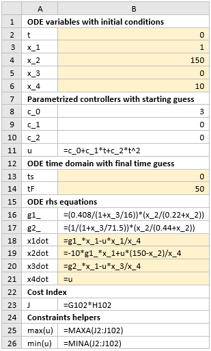
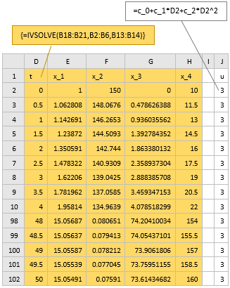
The cost index in this problem is simple and defined by formula B23 by referencing cells G102 and H102 of the solution array which correspond to x3(tF) and x4(tF) respectively. A column of values for the parametrized control u formula is generated in column J as shown in Figure 2. To impose the bound constraint (9) on the control, we demand that the maximum and minimum values of the control vector as computed in B25 and B26 satisfy the appropriate bounds.
We configure Excel Solver to maximize the cost index J, by varying the terminal time tF, and the coefficients B8:B10 subject to the constraints:
H102 <= 200, corresponding to (10)
B25 <= 12, corresponding to (9)
B26 >= -12, corresponding to (9)
The Solver converges in approximately 28 seconds to the result shown in Figure 3, and plotted in Figure 4.
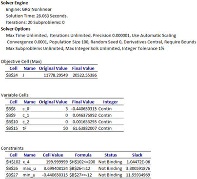
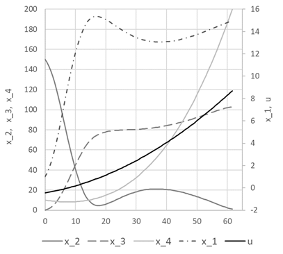
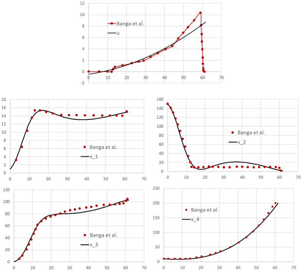
Our achieved maxima for the cost index is at 20522.5 and the terminal time tF is found at approximately 61.64. These values are in very good agreement with the best results reported by Banga et al. [1] at 20839, and 61.17h. Figure 5 shows direct comparison of the states and control trajectories with digitized plot values from Banga et al. The agreement is quite good for the most part for the state variables and the control despite fundamentally different control parametrization and algorithms employed by the two methods. In particular, the control parametrization in [1] is approximated by connected line segments whereas our control is a continuous parabola.
[1] J. R. Banga, E. Balsa-Canto, C. G. Moles, and A. A. Alonso. Dynamic optimization of bioprocesses: efficient and robust numerical strategies. Journal of Biotechnology, 2003.
[2] Ghaddar, C.K. "Rapid Solution of Optimal Control Problems by a Functional Spreadsheet Paradigm: A Practical Method for the Non-Programmer". Math. Comput. Appl. 2018, 23, 54.
Available at: https://www.mdpi.com/2297-8747/23/4/54
[3] Ghaddar, C. K. "Novel Spreadsheet Direct Method for Optimal Control Problems." Math. Comput. Appl., 23, 6, 2018.
Available at: http://www.mdpi.com/2297-8747/23/1/6