
This problem is concerned with planning the 2D motion for a robot from point A (0,0) to point B (1,1), such that to avoid two circular obstacles of radius R2 = 0.1,
centered at (0.4,0.5) and (0.8,1.5), while using the least amount of energy. The two controls for the robot motion are the constant speed, v, and the variable angle (direction),
![]() of the motion. The corresponding optimal control problem has the following form [1]:
of the motion. The corresponding optimal control problem has the following form [1]:
Find ![]() which
which
minimize the energy cost indexs |
|
|---|---|
|
|
(1) |
subject to |
|
|
|
(2) |
|
|
(3) |
with initial conditions |
|
|
|
(4) |
end conditions |
|
|
|
(5) |
and trajectory constraints |
|
|
|
(6) |
|
|
(7) |
We demonstrate next how to employ three calculus function, DERIVXY, QUADXY, and IVSOLVE, to implement a spreadsheet direct solution strategy.
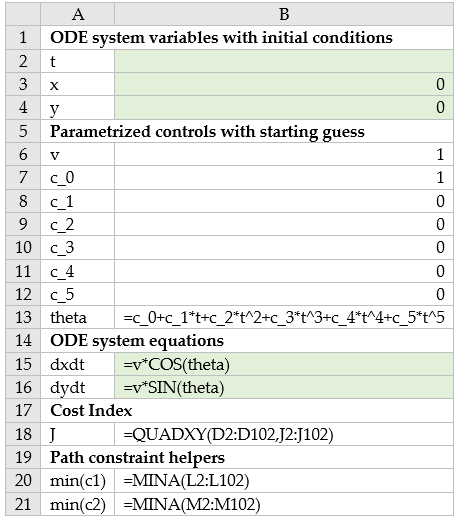
Referring to Figure 1, we parametrize the speed with the variable v in B6,
and parametrize theta with a fifth order polynomial in B13. We obtain an initial solution to the inner initial value problem (2)-(4) by evaluating the
array formula =IVSOLVE(B15:B16, B2:B4, {0,1}) in array D1:F102 partially shown in Figure 2.
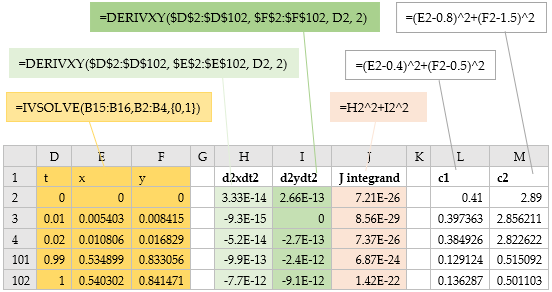
Our next task is to define an analog formula for the cost index (1). The integrand for the cost index depends on ![]() ,
and
,
and ![]() which are not readily available in the obtained solution but we can generate them using
the discrete data differentiator DERIVXY
as shown in columns H and I of Figure 2. For example, to compute
which are not readily available in the obtained solution but we can generate them using
the discrete data differentiator DERIVXY
as shown in columns H and I of Figure 2. For example, to compute ![]() , we start from the formula
, we start from the formula
=DERIVXY($D$2:$D$102, $E$2:$E$102, D2, 2)
in H2 passing in, respectively, the time and x vectors from the IVP solution array, the point of differentiation, and the order of the x derivative to compute.
We then use AutoFill to generate values for all the points in the time vector. (Note that we have locked the first two arguments using Excel $ operator to prevent
these values from being incremented during the AutoFill and allow D2 only to be incremented.)
Values for the integrand expression ![]() are now readily generated in column J
using the generated 2nd derivative values. Finally, the analog formula for the cost index is defined by integrating the integrand column J2:J102 with respect to the time column
D2:D102 as shown in B18 of Figure 1.
are now readily generated in column J
using the generated 2nd derivative values. Finally, the analog formula for the cost index is defined by integrating the integrand column J2:J102 with respect to the time column
D2:D102 as shown in B18 of Figure 1.
The remaining task is to define formulas for the circle avoidance constraints. We generate values for the constraints equations (6) and (7) as shown in columns L and M of Figure 2. To impose the bounds, it is sufficient to require that the minimum values of columns L and M, as computed in B20 and B21 of Figure 1 be greater than or equal to the specified bound.
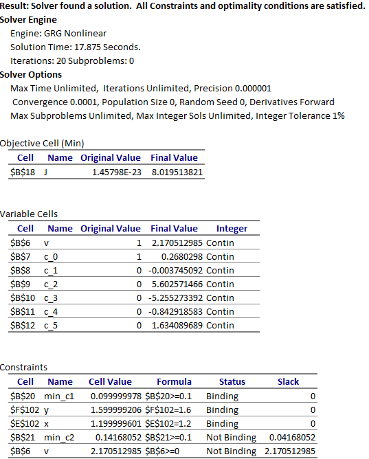
We configure Excel Solver to minimize the cost index, JJ, by varying the speed v, and theta polynomial coefficients B7:B12, subject to the constraints:
v >=0,
E102=1.2, corresponds to (5)
F102=1.6, corresponds to (5)
B20 >=0.1, corresponds to (6)
B21>=0.1, corresponds to (7)
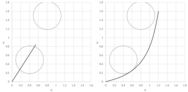
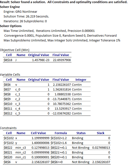
The initial trajectory for the robot based on our starting guess for the controls is shown in Figure 3L. The Solver converges to the low-energy expected solution shown in Figure 3R in approximately 19 seconds with the result shown in Figure 4. The cost index value is found at approximately 8.01.
To make the problem more interesting, we add a 3rd circle obstacle by appending the additional path constraint to the problem:
|
|
(8) |
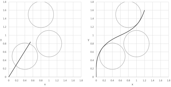
The new configuration and initial trajectory is shown in Figure 5L. The incorporation of (8) into the model setup is straight forward. The solver now converges to the higher energy trajectory shown in Figure 5R at a cost index of approximately 22.69 with the results shown in Figure 6.
[1] R. Bhattacharya. OPTRAGEN 2.0: A MATLAB Toolbox for Optimal Trajectory Generation. Texas A&M University, College Station, TX 77843-3141, USA, Feb 10 2013.
[2] Ghaddar, C.K. "Rapid Solution of Optimal Control Problems by a Functional Spreadsheet Paradigm: A Practical Method for the Non-Programmer". Math. Comput. Appl. 2018, 23, 54.
Available at: https://www.mdpi.com/2297-8747/23/4/54
[3] Ghaddar, C. K. "Novel Spreadsheet Direct Method for Optimal Control Problems." Math. Comput. Appl., 23, 6, 2018.
Available at: http://www.mdpi.com/2297-8747/23/1/6
 .
.