ExcelWorks LLC

Examples 1-4 Workbook

Examples 5-8 Workbook

Optimal Control Problems

An optimal control problem is typically concerned with finding optimal control functions (or policies) that achieve optimal trajectories for a set of controlled differential state variables. The optimal trajectories are decided by a constrained dynamical optimization problem, such that a cost functional is minimized or maximized subject to certain constraints on state variables and the control functions. Mathematically, an optimal control problem may be stated as follows:

Find the control functions and the corresponding state variables which

In the formulation (1)-(5), the generally nonlinear H and G are scalar functions, whereas F, Q, and S are vector-valued functions. Common forms of Q and S are and , respectively. The matrix M in (2) offers an optional coupling of the states' temporal derivatives by a mass matrix which may be singular. If M is singular, the equation system (2) is differential algebraic, or DAE. Furthermore, T, which denotes the final time, may be fixed or free.

Spreadsheet Direct Solution Method with ExceLab

Below, we describe the general steps for employing IVSOLVE and QUADXY with Excel Solver for solving the optimal control problem (1)-(5). To simplify the discussion, we shall assume a single control function, u(t). Extension to multiple controls is straightforward and is demonstrated by the examples. In practice, there are three systematic tasks:

Task 1

The first step is to obtain, with the IVP solver function, IVSOLVE, an initial solution for the underlining IVP (2)-(3) using an appropriately parametrized formula for the control function and initial guesses for the unknown parameters. A continuous control function can be parametrized, for example, by a third-order polynomial with unknown coefficients, such as '=c_0+c_1*t+c_2*t^2+c_3*t^3'. On the other hand, a discontinuous control function can be modeled using the standard IF statement in Excel. For example, a two-stage, constant controller can be defined as follows: '=IF(t<=ts,value1,value2)'. Here ts, value1, and value2 are unknown parameters that would be assigned initial guesses.

Task 2

In the second task we define an analogous objective formula for the cost functional (1). Our strategy is to integrate, using QUADXY, a sampled vector of the integrand expression in (1) using the solution values obtained in Task 1. To accomplish this, in a new column, we generate values for the parametrized control formula evaluated at the solution's output times and, in a second column, we generate values for the integrand expression, using the solution's state variables and generated control values as needed. To define an analogous objective formula for the cost index (1), we employ the discrete data integrator function, QUADXY, to integrate the generated integrand data column versus the solution's output times column. The ordered steps needed to define the objective formula are summarized in Figure 1.

Task 3

The last task is to configure and run Excel's NLP Solver. The NLP Solver can be configured to minimize or maximize an objective formula by changing design variables, subject to defined constraints. The design variables are the unknown parameters which are assigned initial guesses in Task 1. The constraints (4) and (5) are added directly in the Solver's dialog. Simple equality end conditions on state variables are added by referencing the corresponding cells in the solution output as illustrated in Figure 1. Bound constraints on state variables or controls are easily imposed with the aid of Excel's MAXA() and MINA() math functions which compute the maximum and minimum values of a vector. Concrete examples are presented in the next section.

How It Works

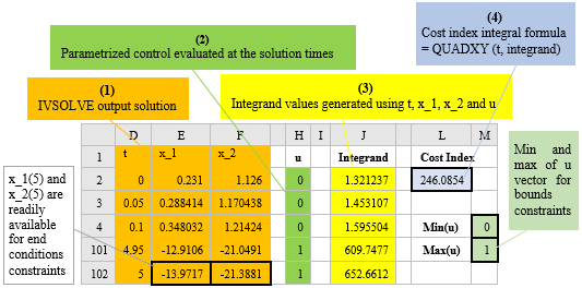
Excel maintains dependency hierarchy, and updates all information whenever a change occurs. Any modification to the design parameters by Excel Solver triggers reevaluation of the inner IVSOLVE solution, the dependent control and integrand columns, the objective, and any constraint formulas in the proper order. Excel Solver always receives up-to-date values for the objective and constraints whenever it alters the design variables values.