
The second example represents an unconstrained optimal control problem in the fixed interval t ∈ [-1, 1] , but with highly nonlinear equations. The mathematical problem is stated as follows:
|
Minimize |
|
|---|---|
|
|
(1) |
|
subject to |
|
|
|
(2) |
|
|
(3) |
|
|
(4) |
The spreadsheet model for the initial value problem (2)-(4) with a parametrized control function using a third-order polynomial is shown in Table 1.
| A | B | |
| 1 | ODE variables | |
|---|---|---|
| 2 | t | -1 |
| 3 | x_1 | 0.05 |
| 4 | x_2 | 0 |
| 5 | Parametrized control formula | |
| 6 | c_0 | 1 |
| 7 | c_1 | 0 |
| 8 | c_2 | 1 |
| 9 | c_3 | 0 |
| 10 | u | =c_0+c_1*t+c_2*t^2+c_3*t^3 |
| 11 | ODE rhs equations | |
| 12 | x1dot | =0.78*(-2*(x_1+0.25)+(x_2+0.5)*EXP(25*x_1/(x_1+2))-(x_1+0.25)*u)/2 |
| 13 | x2dot | =0.78*(0.5-x_2-(x_2+0.25)*EXP(25*x_1/(x_1+2)))/2 |
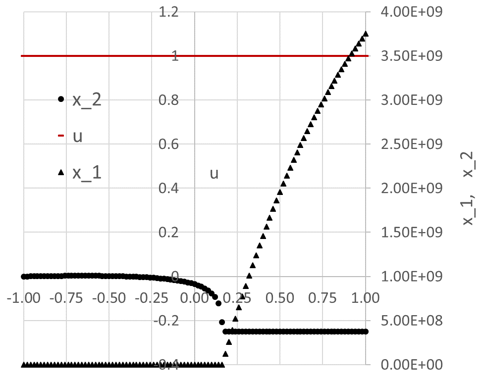
The initial solution to the IVP is obtained by evaluating the array formula =IVSOLVE(B12:B13, B2:B4, {-1,1})
in an allocated array E2:G103, which is shown partially in Table 2 and plotted in Figure 1.
Clearly, our initial guess for the control coefficients B6:B9 is not good, since the solution exhibits instabilities at larger time values.
The control and integrand vectors, needed to construct the objective formula for the cost index (1), are
generated in columns I and K from the formulas I3 and K3, listed in Table 3.
The objective (1) is defined by the formula N3 using QUADXY with an initial cost of 1.92 x 10¹⁸.
| E | F | G | H | I | J | K | |
| 1 | IVP Solution | ||||||
|---|---|---|---|---|---|---|---|
| 2 | t | x_1 | x_2 | u | Integrand | Cost functional | |
| 3 | -1.00 | 0.05 | 0 | 1 | 0.1025 | Objective | 1.92396E+18 |
| 4 | -0.98 | 0.050163 | 0.000305 | 1 | 0.102516 | ||
| 5 | -0.96 | 0.050341 | 0.000596 | 1 | 0.102535 | ||
| 100 | 0.94 | 3.59E+09 | -0.25 | 1 | 1.29E+19 | ||
| 101 | 0.96 | 3.64E+09 | -0.25 | 1 | 1.33E+19 | ||
| 102 | 0.98 | 3.7E+09 | -0.25 | 1 | 1.37E+19 | ||
| 103 | 1.00 | 3.75E+09 | -0.25 | 1 | 1.41E+19 | ||
| Purpose | Cell | Formula |
|---|---|---|
| Initial value problem solution | E2:G103 | =IVSOLVE(B12:B13, B2:B4, {-1,1}) |
| AutoFill formula for control values | I3 | =c_0+c_1*E3+c_2*E3^2+c_3*E3^3 |
| AutoFill formula for integrand values | K3 | =F3^2+G3^2+0.1*I3^2 |
| Objective | N3 | =0.78*QUADXY(E3:E103, K3:K103)/2 |
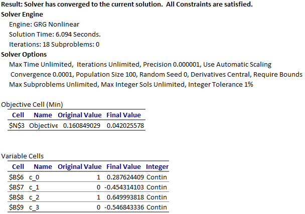
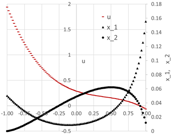
We configure Excel Solver to minimize the objective formula N3 by varying the control parameters B6:B9 with no added constraints. Despite the bad initial values for the control parameters, the Solver reported a feasible solution in about 2 seconds with the Answer Report shown in Figure 2. The optimal trajectories for the system variables are plotted in Figure 3.
[1] Elnagar, G.; Kazemi, M.A. Pseudospectral Chebyshev Optimal Control of Constrained Nonlinear Dynamical Systems. Comput. Optim. Appl. 1998, 11, 195-217.
[2] Ghaddar, C. K. "Novel Spreadsheet Direct Method for Optimal Control Problems." Math. Comput. Appl., 23, 6, 2018.
Available at: http://www.mdpi.com/2297-8747/23/1/6
[3] Ghaddar, C.K. "Rapid Solution of Optimal Control Problems by a Functional Spreadsheet Paradigm: A Practical Method for the Non-Programmer". Math. Comput. Appl. 2018, 23, 54.
Available at: https://www.mdpi.com/2297-8747/23/4/54