
This example is concerned with finding the shape u(t) of a chain of length L=4 suspended between two points, such that its total energy is minimized. We state the problem as described in [1]:
Find u(t) which
|
minimizes the total energy cost index |
|
|---|---|
|
|
(1) |
|
subject to the chain length constraint |
|
|
|
(2) |
|
and the end conditions |
|
|
|
(3) |
|
|
(4) |
In [1], the best cost index was found at 5.06852 starting from a quadratic approximation.
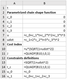
Referring to Figure 1, we setup the model in Excel using the named variables in column A. We parametrize the shape function u(t) using a 3rd
order polynomial. In B15 and B16, we define formulas for the initial and final values, u(0) and u(1) by evaluating B7
at t=0 and t=1. We also define in B8 a formula for the shape function derivative, ![]() by differentiating B7 with respect to t.
We define the cost index integral (1), by using the integration function QUADF to integrate
by differentiating B7 with respect to t.
We define the cost index integral (1), by using the integration function QUADF to integrate
![]() which is defined in B10. Likewise, we use QUADF,
to define the constraint integral (2) as shown in B14. This completes the model needed to run Excel Solver.
which is defined in B10. Likewise, we use QUADF,
to define the constraint integral (2) as shown in B14. This completes the model needed to run Excel Solver.
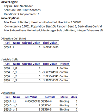
We configure Excel Solver to minimize the objective J, by varying the parameters c_0, c_1, c_2 and c_3, subject to the constraints:
I_c=4, corresponding to (2)
u_0=1, corresponding to (3)
u_1=3, corresponding to (4).
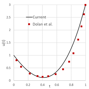
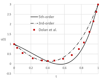
The Solver converges, starting from a zero guess for the parameters in less than a second to the result shown in Figure 2 with a final cost index of 5.0751. The optimal shape function u(t) is plotted in Figure 3 together with digitally-read values from the plot published in [1].
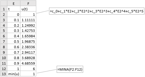
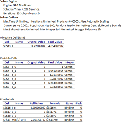
To demonstrate the effect of the control parametrization order on the result, we try next, a 5th-order polynomial approximation to the shape function u(t), but also append the problem with one additional constraint:
|
|
(5) |
Incorporating (5) into the spreadsheet model is accomplished as follows. In a new column we generate a vector of time values from 0 to 1 and a corresponding vector for the parametrized shape formula as shown in Figure 4. We compute the minimum value of the shape vector in F13. To impose (5), we add the additional constraint F13 ≥ 0 to Excel Solver.
Running Excel Solver with the added constraint yields a lower cost index of 4.654. The new result is shown in Figure 5 and plotted in Figure 6.
[1] E.D. Dolan and J.J. More. Benchmarking optimization software with cops. Technical report, ARGONNE NATIONAL LABORATORY, 9700 South Cass Avenue, Argonne, Illinois 60439, January 2001.
[2] Ghaddar, C.K. "Rapid Solution of Optimal Control Problems by a Functional Spreadsheet Paradigm: A Practical Method for the Non-Programmer". Math. Comput. Appl. 2018, 23, 54.
Available at: https://www.mdpi.com/2297-8747/23/4/54
[3] Ghaddar, C. K. "Novel Spreadsheet Direct Method for Optimal Control Problems." Math. Comput. Appl., 23, 6, 2018.
Available at: http://www.mdpi.com/2297-8747/23/1/6