
The third example represents the problem of transferring containers, driven by a hoist motor and a trolley drive motor, from a ship to a cargo truck. The goal is to minimize the swing during and at the end of the transfer. The mathematical optimal control problem is described by (1)-(13). The problem is nonlinear with six state variables and two controllers subject to multiple final and bound constraints.
|
Minimize |
|
|---|---|
|
|
(1) |
|
subject to |
|
|
|
(2) |
|
|
(3) |
|
|
(4) |
|
|
(5) |
|
|
(6) |
|
|
(7) |
|
Initial conditions: |
|
|
|
(8) |
|
Final conditions: |
|
|
|
(9) |
|
Bounds: |
|
|
|
(10) |
|
|
(11) |
|
|
(12) |
|
|
(13) |
Following the same procedure as that in the previous examples, we define the model for the IVP (2)-(8) using third-order parametrized polynomial control functions as shown in Table 1. Initial values and guesses are assigned to the state variables and unknown parametrization coefficients as shown in the table.
| A | B | C | D | |
| 1 | ODE variables | |||
| 2 | t | 0 | ||
| 3 | x_1 | 0 | ||
| 4 | x_2 | 22 | ||
| 5 | x_3 | 0 | ||
| 6 | x_4 | 0 | ||
| 7 | x_5 | -1 | ||
| 8 | x_6 | 0 | ||
| 9 | Parametrized controls formulas | |||
| 10 | c_0 | 1 | d_0 | 1 |
| 11 | c_1 | 1 | d_1 | 1 |
| 12 | c_2 | -5 | d_2 | -5 |
| 13 | c_3 | -5 | d_3 | -5 |
| 14 | u_1 | =c_0+c_1*t+c_2*t^2+c_3*t^3 | ||
| 15 | u_2 | =d_0+d_1*t+d_2*t^2+d_3*t^3 | ||
| 16 | ODE rhs equations | |||
| 17 | x1dot | =9*x_4 | ||
| 18 | x2dot | =9*x_5 | ||
| 19 | x3dot | =9*x_6 | ||
| 20 | x4dot | =9*(u_1+x_3) | ||
| 21 | x5dot | =9*u_2 | ||
| 22 | x6dot | =9*(u_1+27.0756*x_3+2*x_5*x_6)/x_2 | ||
Table 2 shows a partial listing of the initial solution obtained by evaluating the array formula =IVSOLVE(B17:B22, B2:B8, {0,1})
in array F2:L103, along with the generated control columns for u_1, u_2, and the integrand expression using the corresponding formulas listed in Table 3.
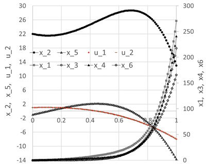
The initial system trajectories are plotted in Figure 1.
Next, we defined the objective formula, S3, corresponding to the cost index (17) as shown in Table 3, in which the data integrator QUADXY was used to integrate the generated integrand expression values. The objective formula evaluated to an initial value of 24,229.22793. Table 3 also lists a number of aid formulas which compute the minimum and maximum values for the state variables x_4 and x_5 and the generated control columns. These aid formulas were used to define the bound constraints for the NLP Solver.
| F | G | H | I | J | K | L | N | O | P | R | S | |
| 1 | IVP Solution | |||||||||||
|---|---|---|---|---|---|---|---|---|---|---|---|---|
| 2 | t | x_1 | x_2 | x_3 | x_4 | x_5 | x_6 | u_1 | u_2 | Integrand | ||
| 3 | 0 | 0 | 22 | 0 | 0 | -1 | 0 | 1 | 1 | 0 | Objective | 24229.22793 |
| 4 | 0.01 | 0.004063 | 21.91406 | 0.000185 | 0.09044 | -0.90957 | 0.00411 | 1.009495 | 1.009495 | 1.69E-05 | ||
| 5 | 0.02 | 0.016305 | 21.8363 | 0.000742 | 0.181723 | -0.81832 | 0.008285 | 1.01796 | 1.01796 | 6.92E-05 | Constraints | |
| 6 | 0.03 | 0.036797 | 21.76679 | 0.001679 | 0.273786 | -0.72636 | 0.012569 | 1.025365 | 1.025365 | 0.000161 | max(u1) | 1.045855 |
| 101 | 0.98 | 230.6731 | 15.34798 | 189.5472 | 205.5287 | -12.3527 | 147.8948 | -7.52796 | -7.52796 | 57801.01 | ||
| 102 | 0.99 | 249.9267 | 14.20542 | 203.2503 | 222.511 | -13.0407 | 156.6717 | -7.762 | -7.762 | 65856.72 | ||
| 103 | 1 | 270.7634 | 13 | 217.7568 | 240.7409 | -13.75 | 165.7417 | -8 | -8 | 74888.35 | ||
| Purpose | Cell | Formula |
|---|---|---|
| Initial value problem solution | F2:L103 | =IVSOLVE(B17:B22, B2:B8, {0,1}) |
| AutoFill formula for u_1 control values | N3 | =c_0+c_1*F3+c_2*F3^2+c_3*F3^3 |
| AutoFill formula for u_2 control values | O3 | =d_0+d_1*F3+d_2*F3^2+d_3*F3^3 |
| AutoFill formula for integrand values | P3 | =I3^2+L3^2 |
| Objective Formula | S3 | =4.5*QUADXY(F3:F103, P3:P103) |
| u_1 column max value | S6 | =MAXA(N3:N103) |
| u_1 column min value | S7 | =MINA(N3:N103) |
| u_2 column max value | S8 | =MAXA(O3:O103) |
| u_2 column min value | S9 | =MINA(O3:O103) |
| x_4 column max value | S10 | =MAXA(J3:J103) |
| x_4 column min value | S11 | =MINA(J3:J103) |
| x_5 column max value | S12 | =MAXA(K3:K103) |
| x_5 column min value | S13 | =MINA(K3:K103) |
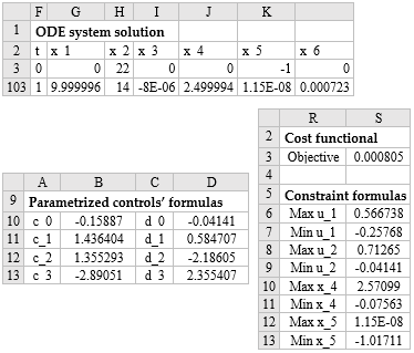
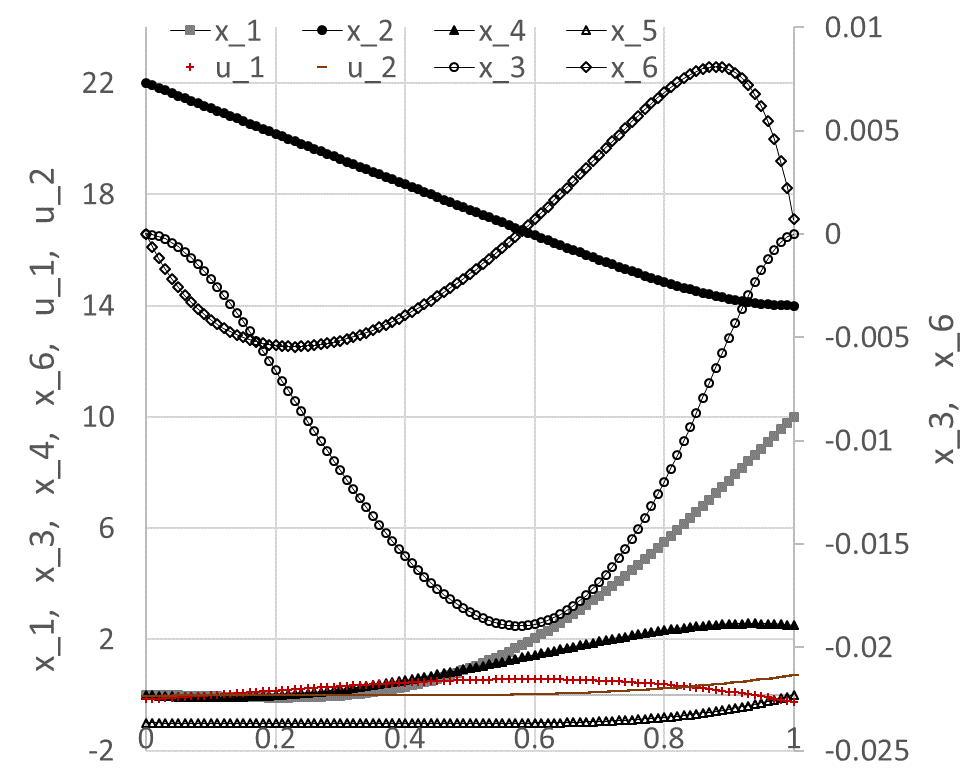
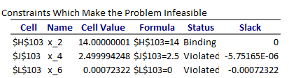
We configured Excel Solver to minimize the objective formula S3 by varying the controls' coefficients B10:B14 and D10:D14 subject to the constraints listed in Table 4. The Solver spun for a few seconds, then reported that it did not find a feasible solution when, in fact, it already had, judging by the best-found solution results shown partially in Figure 2 and plotted in Figure 3. The solution indicates that all constraints were satisfied within a reasonable tolerance of 1x10⁻⁵, except for x_6(1), which was satisfied within a tolerance of 1x10⁻³. This is verified by the feasibility report generated by the Solver, and shown in Figure 4.
| Formula | Constraint |
|---|---|
| G103 = 10 | |
| H103 = 14 | |
| I103 = 0 | |
| J103 = 2.5 | |
| K103 = 0 | |
| L103 = 2.5 | |
| S10 ≤ 2.5 | (12) |
| S11 ≥ -2.5 | |
| S12 ≤ 1 | (13) |
| S13 ≥ -1 | |
| S6 ≤ 2.83374 | (10) |
| S7 ≥ -2.83374 | |
| S8 ≤ 0.71265 | (11) |
| S9 ≥ -0.80865 |
[1] Elnagar, G.; Kazemi, M.A. Pseudospectral Chebyshev Optimal Control of Constrained Nonlinear Dynamical Systems. Comput. Optim. Appl. 1998, 11, 195-217.
[2] Ghaddar, C. K. "Novel Spreadsheet Direct Method for Optimal Control Problems." Math. Comput. Appl., 23, 6, 2018.
Available at: http://www.mdpi.com/2297-8747/23/1/6
[3] Ghaddar, C.K. "Rapid Solution of Optimal Control Problems by a Functional Spreadsheet Paradigm: A Practical Method for the Non-Programmer". Math. Comput. Appl. 2018, 23, 54.
Available at: https://www.mdpi.com/2297-8747/23/4/54