Example solving a minimum time orbit transfer problem in Excel.

Minimum Time Orbit Transfer Problem

The fourth example describes a minimum time orbit transfer problem . The goal is to minimize the transfer time of a constant thrust rocket between the orbits of Earth and Mars, and to determine the optimal thrust angle control. The original free-time mathematical problem is stated as follows:

Minimize
	(1)
subject to
	(2)
	(3)
	(4)
with initial conditions
	(5)
and final conditions
	(6)

In [1], the original problem was transformed into a fixed time domain [-1, 1]. The corresponding value for the transfer time, t_F , was reported at 3.31873 using ninth-degree Chebyshev polynomial approximations. Here, we solve the original free-time problem as stated in (1)-(6).

Spreadsheet Model

Referring to Table 1, the initial value problem (2)-(5) is modeled using a third-order parametrized polynomial approximation for u(t) with zero initial guess for the unknown coefficients. Since t_F is free, it is assigned its own variable, B13 with an initial guess of 10.

Table 1
	A	B
1	ODE variables
2	t	0
3	x_1	1
4	x_2	0
5	x_3	1
6	System Parameters
7	gamma	1
8	R0	0.1405
9	m0	1
10	mdot	-0.07487
11	Time Domain
12	t0	0
13	tF	10
14	Parametrized controller formula
15	c_0	0
16	c_1	0
17	c_2	0
18	c_3	0
19	u	=c_0+c_1t+c_2t^2+c_3*t^3
20	ODE rhs equations
21	x1dot	=x_2
22	x2dot	=x_3^2/x_1-gamma/x_1^2+R0SIN(u)/(m0+mdott)
23	x3dot	=-x_2x_3/x_1+R0COS(u)/(m0+mdot*t)

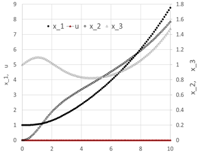
We obtain the initial solution by evaluating the array formula =IVSOLVE(B21:B23, B2:B5, B12:B13) in array E2:H103 shown partially in Table 2 along with the generated control column and the initial objective value using the formulas listed in Table 3. Note that the third argument to the IVSOLVE formula is the variable time domain [0, t_F] which is represented by the range B12:B13. The initial trajectories for the system are plotted in Figure 1.

Table 2
	E	F	G	H	I	J	K
1	IVP Solution
2	t	x_1	x_2	x_3	u	Cost functional
3	0.00	1	0	1	0	Objective	10
4	0.10	1.000047	0.001413	1.014055	0
5	0.20	1.000378	0.005681	1.027927	0
6	0.30	1.001278	0.012807	1.041313	0
7	0.40	1.003034	0.02276	1.053905	0
100	9.70	8.305837	1.499819	1.391005	0
101	9.80	8.456923	1.521927	1.417734	0
102	9.90	8.610249	1.544573	1.445546	0
103	10.00	8.765865	1.567783	1.474497	0

Table 3: formulas used to generate values shown in Table 2
Purpose	Cell	Formula
Initial value problem solution	`E2:H103`	`=IVSOLVE(B21:B23, B2:B5, B12:B13)`
AutoFill formula for control values	`J3`	`=c_0+c_1E3+c_2E3^2+c_3*E3^3`
Objective formula	`L3`	`=t_F`

Results and Discussion

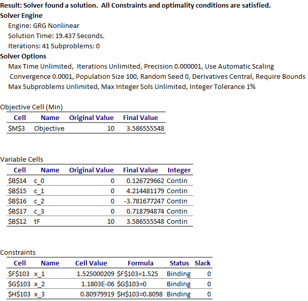
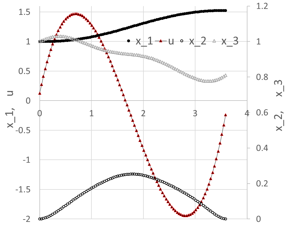
We configure Excel Solver to minimize the objective formula L3 by varying the end time t_F, B13, and the control coefficients B15:B18, subject to the end point equality constraints on the state variables (6). The constraints are added directly into the Solver dialog by referencing the corresponding cells in the last row of the IVSOLVE solution array in Table 2. The Solver reported, in under 20 seconds, the feasible solution shown in the Answer Report of Figure 2. The minimum orbit time, t_F , was found to be 3.58656. This compares reasonably well to the value reported in [1] at 3.31873 using ninth-degree Chebyshev polynomial approximations. The optimal trajectories are plotted in Figure 3.

References

[1] Elnagar, G.; Kazemi, M.A. Pseudospectral Chebyshev Optimal Control of Constrained Nonlinear Dynamical Systems. Comput. Optim. Appl. 1998, 11, 195-217.

[2] Ghaddar, C. K. "Novel Spreadsheet Direct Method for Optimal Control Problems." Math. Comput. Appl., 23, 6, 2018.
Available at: http://www.mdpi.com/2297-8747/23/1/6

[3] Ghaddar, C.K. "Rapid Solution of Optimal Control Problems by a Functional Spreadsheet Paradigm: A Practical Method for the Non-Programmer". Math. Comput. Appl. 2018, 23, 54.
Available at: https://www.mdpi.com/2297-8747/23/4/54

ExcelWorks LLC

Minimum Time Orbit Transfer Problem

Spreadsheet Model

Results and Discussion

References